src/README.trace
Built-in profiling
Functions marked with the trace keyword can be automatically instrumented to keep a record of how much time is spent within each of these functions. In addition the time spent in events can also be automatically tracked.
To activate built-in profiling the TRACE macro needs to be set with a value larger than 1 for example using
CFLAGS=-DTRACE=2 make test.tstor
qcc -DTRACE=2 test.c -o test -lmAfter execution, the program will then produce a report on standard output looking like
cat test/out
...
   calls    total     self   % total   function
    2193     1.09     1.09     43.2%   boundary():/home/popinet/basilisk-octree/src/grid/cartesian-common.h:268
     874     1.28     0.96     38.0%   update_saint_venant():/home/popinet/basilisk-octree/src/saint-venant.h:272
     438     0.60     0.19      7.5%   adapt():bump2D.c:65
      18     0.19     0.18      7.2%   output_field():/home/popinet/basilisk-octree/src/output.h:100
     874     0.41     0.05      2.1%   advance_saint_venant():/home/popinet/basilisk-octree/src/saint-venant.h:100
     438     0.02     0.02      0.7%   logfile():bump2D.c:23
  147456     0.01     0.01      0.5%   interpolate():/home/popinet/basilisk-octree/src/grid/cartesian-common.h:581
       1     2.52     0.01      0.3%   run():/home/popinet/basilisk-octree/src/predictor-corrector.h:80
       9     0.20     0.00      0.2%   outputfile():bump2D.c:49
       3     0.00     0.00      0.1%   init_grid():/home/popinet/basilisk-octree/src/grid/tree.h:1527
       1     0.00     0.00      0.1%   defaults():/home/popinet/basilisk-octree/src/predictor-corrector.h:45
       1     0.00     0.00      0.0%   init_0():bump2D.c:18
       1     0.00     0.00      0.0%   init():/home/popinet/basilisk-octree/src/saint-venant.h:310
       1     0.00     0.00      0.0%   defaults_0():/home/popinet/basilisk-octree/src/saint-venant.h:299
The first column is the number of times the function was called. The second column is the total time spent within the function (including any calls to other functions). The third column is the time spent within the function, excluding any time spent within called functions which are traced, i.e. this is really the time spent executing instructions belonging to the function. The “self” time is what is used to rank the function and to report the percentage of the total time indicated in the fourth column. The fifth column gives the name of the traced function, the file it belongs to and the line number corresponding to the point where the function returned (i.e. the end of the function, not the start).
For this example (the bump2D test case), we see that we spent 1.09 seconds (43.2% of the total) applying boundary conditions (this is mostly coarse/fine interpolations due to adaptive refinement), 0.96 seconds (38%) doing actual work (in the Saint-Venant solver), 0.19 seconds (7.5%) doing mesh adaptation, and so on. We also see that output_field() used a significant amount of the total (7.2%) i.e. we could easily speed up the calculation (a bit) by outputting less often (i.e. less than 18 times).
Graphing tools
It is sometimes useful to monitor the evolution with time of how much time is taken by each function. This can be done by adding something like:
#if TRACE > 1
event profiling (i += 20) {
  static FILE * fp = fopen ("profiling", "w");
  trace_print (fp, 1);
}
#endif
where argument 1 specifies that only functions taking more than one percent of runtime should be displayed. The profiling file will contain records looking like the above but measured between successive calls to the trace_print() function (not over the entire program runtime). These data can be conveniently displayed using
gnuplot> load ("< awk -f $BASILISK/trace.awk < profiling");which will display a graph looking like:
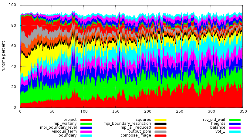
Output of the trace.awk profiling script
The functions are arranged in decreasing order of runtime (for example here the project() function takes the largest proportion of the runtime, followed by mpi_waitany() etc.). The horizontal axis is the time, where the units are the number of outputs of the profiling() event above.
This can also be automated using continuous monitoring.