shoal-ml.c

Periodic wave propagation over an ellipsoidal shoal

Periodic wave propagation over an ellipsoidal shoal

We follow Lannes and Marche, 2014 and try to reproduce the experiment of Berkhoff et al, 1982. The numerical wave tank is 25² metres and periodic waves are generated on the left-hand side and are damped on the right-hand side.

#include "grid/multigrid.h"
#if ML
# include "layered/hydro.h"
# include "layered/nh.h"
# include "layered/remap.h"
# include "layered/perfs.h"
#else // !ML
# include "green-naghdi.h"
#endif

int main()
{
  X0 = -10;
  L0 = 25 [1];
  Y0 = -L0/2.;
  G = 9.81;

#if ML
  N = 512;
  nl = 2;
  CFL_H = 1;
#else // Green-Naghdi

The Green–Naghdi solver is significantly more dissipative, so we have to turn off limiting and increase resolution.

  N = 1024;
  gradient = NULL;
#endif
  
  run();
}

We declare a new field to store the maximum wave amplitude.

scalar maxa[];

Periodic waves with period one second are generated on the left-hand-side. We tune the amplitude of the “radiation” condition to match that of the experiment as measured by wave gauges. This is different for the two solvers, in particular because of the different spatial resolutions. It would be nice to devise a resolution-independent wave generator.

double T0 = 1.;
#if ML
double A = 0.06;
#else
double A = 0.042; // 0.049
#endif

event init (i = 0)
{
  u.n[left]  = - radiation (A*sin(2.*pi*t/T0));
  u.n[right] = + radiation (0);

The bathymetry is an inclined and skewed plane combined with an ellipsoidal shoal.

set term @PNG enhanced size 640,640 font ",8"
set output 'bathy.png'
set pm3d map
set palette defined ( 0 0 0 0.5647, 0.125 0 0.05882 1, 0.25 0 0.5647 1, \
                      0.375 0.05882 1 0.9333, 0.5 0.5647 1 0.4392,	  \
                      0.625 1 0.9333 0, 0.75 1 0.4392 0,		  \
                      0.875 0.9333 0 0, 1 0.498 0 0 )
set size ratio -1
set xlabel 'x (m)'
set ylabel 'y (m)'
splot [-10:12][-10:10]'end' u 1:2:4 w pm3d t ''
# we remove the large border left by gnuplot using ImageMagick
! mogrify -trim +repage bathy.png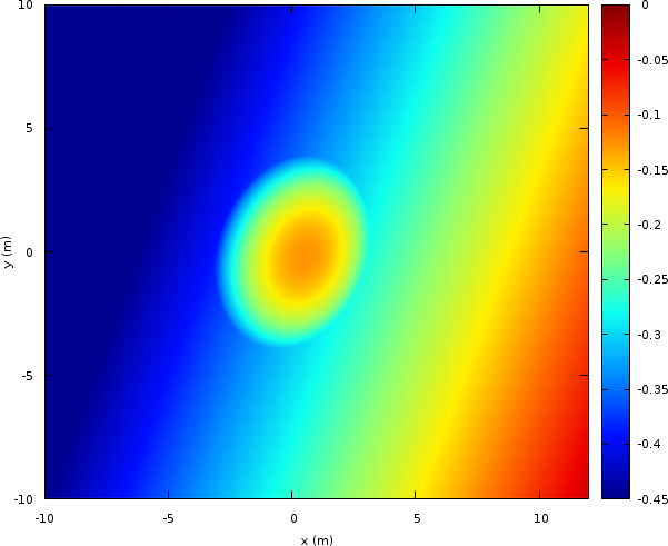

Bathymetry (script)

  double h0 = 0.45;
  double cosa = cos (20.*pi/180.), sina = sin (20.*pi/180.);
  foreach() {
    double xr = x*cosa - y*sina, yr = x*sina + y*cosa;
    double z0 = xr >= -5.82 ? (5.82 + xr)/50. : 0.;
    double zs = sq(xr/3.) + sq(yr/4.) <= 1. ?
      -0.3 + 0.5*sqrt(1. - sq(xr/3.75) - sq(yr/5.)) : 0.;
    zb[] = z0 + zs - h0;
#if ML
    foreach_layer()
      h[] = max(-zb[], 0.)*beta[point.l];
#else
    h[] = max(-zb[], 0.);
#endif
    maxa[] = 0.;
  }
}

To implement an absorbing boundary condition, we add an area for x > 12 for which quadratic friction increases linearly with x.

event friction (i++) {
  double b = 2. [-1];
  foreach() 
    if (x > 12.) {
      double a = h[] < dry ? HUGE : 1. [0] + b*(x - 12.)*dt*norm(u)/h[];
#if ML
      foreach_layer()
#endif
	foreach_dimension()
	  u.x[] /= a;
    }
}

Optionally, we can make a “stroboscopic” movie of the wave field. This is useful to check the amount of waves reflected from the outflow.

#if 0
event movie (t += 1) {
  output_ppm (eta, min = -0.04, max = 0.04, n = 512);
}
#endif

After the wave field is established (t >= 40) we record the maximum wave amplitude.

event maximum (t = 40; i++) {
  foreach()
    if (fabs(eta[]) > maxa[])
      maxa[] = fabs(eta[]);
}

At the end of the simulation, we output the maximum wave amplitudes along the cross-sections corresponding with the experimental data.

event end (t = 50) {
  FILE * fp = fopen ("end", "w");
  output_field ({eta,zb,maxa}, fp, linear = true);
  FILE * fp2 = fopen ("section2", "w");
  FILE * fp5 = fopen ("section5", "w");
  FILE * fp7 = fopen ("section7", "w");
  for (double y = -10.; y <= 10.; y += 0.02) {
    fprintf (fp2, "%g %g\n", y, interpolate (maxa, 3., y));
    fprintf (stderr, "%g %g\n", y, interpolate (maxa, 5., y));
    fprintf (fp5, "%g %g\n", y, interpolate (maxa, 9., y));
  }
  for (double x = -10.; x <= 10.; x += 0.02)
    fprintf (fp7, "%g %g\n", x, interpolate (maxa, x, 0.));
}

set output 'snapshot.png'
a0 = 0.026
splot [-10:12][-10:10]'end' u 1:2:($3/a0) w pm3d t ''
! mogrify -trim +repage snapshot.png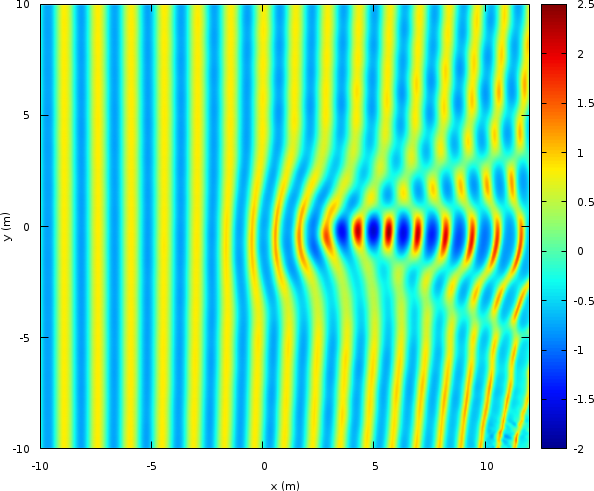

Instantaneous wave field at t=50 (script)

set output 'maxa.png'
set label 1 "section 2" at 2.5,-6,1 rotate front
set label 2 "section 3" at 4.5,-6,1 rotate front
set label 3 "section 5" at 8.5,-6,1 rotate front
set label 4 "section 7" at -3,0.5,1 front
splot [-10:12][-10:10]'end' u 1:2:($5/a0) w pm3d t '', \
 '-' w l lt -1 t ''
3 -10 1
3 10 1


5 -10 1
5 10 1


9 -10 1
9 10 1


-10 0 1
10 0 1
e
unset label
! mogrify -trim +repage maxa.png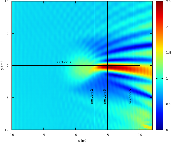

Maximum wave amplitude (script)

The results are comparable to Lannes and Marche, 2014, Figure 19, but we have to use a higher resolution (1024² for the Green–Naghdi solver instead of 300²) because our numerical scheme is only second order (versus 4th order).

reset
set term svg enhanced size 640,480 font ",10"
set multiplot layout 2,2
set key top left
set xlabel 'y (m)'
set ylabel 'a_{max}/a_{0}'
set yrange [0:2.5]
plot [-5:5] '../section-2' pt 7 lc -1 t '', \
          'section2' u (-$1):($2/a0) w l lc 1 lw 2 t 'section 2'
plot [-5:5] '../section-3' pt 7 lc -1 t '', \
     'log' u (-$1):($2/a0) w l lc 1 lw 2 t 'section 3'
plot [-5:5] '../section-5' pt 7 lc -1 t '', \
     'section5' u (-$1):($2/a0) w l lc 1 lw 2 t 'section 5'
set xlabel 'x (m)'
plot [0:10] '../section-7' pt 7 lc -1 t '', \
     'section7' u 1:($2/a0) w l lc 1 lw 2 t 'section 7'
unset multiplot

Comparison of the maximum wave height with the experimental data (symbols) along various cross-sections (script)