/**
# Overflow

This test case was designed by [Ilicak et al., 2012](#ilicak2012),
section 4, to investigate the mixing properties of numerical schemes
in the case of "overflow" i.e. a denser fluid flowing down a sill or
continental slope.

Note that the test case is largely qualitative and is in particular
very sensitive to various sources of dissipation, including bottom
boundary conditions etc.

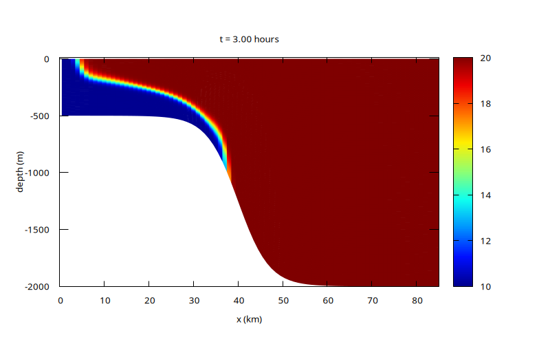
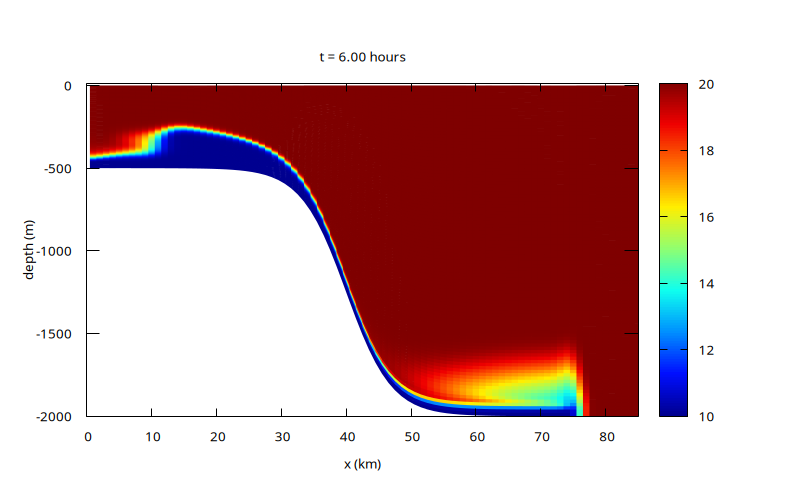
The evolution of the "temperature"/density field is illustrated in the
sequence below. The cool/dense fluid to the left is released at the
top of the slope and flows down. Although no explicit temperature
diffusion is prescribed, numerical diffusion leads to the formation of
a diffused plume in regions of high shear (the "head" of the flow).

![Animation of the temperature field](overflow/movie.mp4)

The figures at $t=3$ and $t=6$ hours below agree closely with Figure
4.k and 4.l of [Petersen et al, 2015](#petersen2015).

<table>
<tr><td>
![$t=3$ hours](overflow/T-3.png){ width=100% }
</td><td>
![$t=6$ hours](overflow/T-6.png){ width=100% }
</td></tr>
</table>

The amount of mixing can be measured by looking at the evolution of
the Reference (or Resting) Potential Energy (RPE) as proposed by
[Ilicak et al, 2012](#ilicak2012). In the ideal case without any
numerically-induced mixing, the RPE should be conserved.

~~~gnuplot Evolution of the normalised reference potential energy
set xlabel 'Time (hours)'
set ylabel '(RPE - RPE(0))/RPE(0) x 10^5'
hour = 3600.
set xrange [0:12]
plot 'log' u ($1/hour):(-$3/$4*1e7) w l t ''
~~~

~~~gnuplot Evolution of the average rate of change of the reference potential energy
set ylabel 'dRPE/dt (Watts/m^2)'
set logscale y
L0 = 256e3
plot 'log' u ($1/hour):(abs($3)/$1/L0) w l t ''
~~~

~~~gnuplot Evolution of the Available Potential Energy (APE = PE - RPE).
set ylabel 'APE (Joules)'
unset logscale y
plot 'log' every 1 u ($1/hour):($5-$3) w l t ''
~~~

~~~gnuplot Evolution of the Kinetic Energy.
set ylabel 'KE (Joules)'
plot 'log' every 1 u ($1/hour):6 w l t ''
~~~

~~~gnuplot Evolution of the Total Energy KE + APE.
set ylabel 'Total Energy (Joules)'
unset logscale
plot 'log' every 10 u 1:($5-$3+$6) w l t ''
~~~

## Non-diffusive interface

This is the same setup but using a vertical remapping which preserves
the sharp temperature/density interface (i.e. the interface is treated
in a Lagrangian manner while the other layers are "Eulerian"). Note
that this is different from the two-layers isopycnal run of [Petersen
et al, 2015](#petersen2015) since here 20 layers are used (10 in each
"phase"), and so the vertical velocity profile is resolved.

![Animation of the temperature field](overflow-isopycnal/movie.mp4)

<table>
<tr><td>
![$t=3$ hours](overflow-isopycnal/T-3.png){ width=100% }
</td><td>
![$t=6$ hours](overflow-isopycnal/T-6.png){ width=100% }
</td></tr>
</table>

In the absence of spurious numerical diffusion, the evolution is much
faster and the front propagates much further.

As expected the resting potential energy is conserved to within
machine accuracy.

~~~gnuplot Evolution of the normalised reference potential energy
set xlabel 'Time (hours)'
set ylabel '(RPE - RPE(0))/RPE(0) x 10^5'
hour = 3600.
set xrange [0:12]
plot '../overflow-isopycnal/log' u ($1/hour):(-$3/$4*1e7) w l t ''
~~~

## References

~~~bib
@article{ilicak2012,
title = {Spurious dianeutral mixing and the role of momentum closure},
journal = {Ocean Modelling},
volume = {45-46},
pages = {37-58},
year = {2012},
issn = {1463-5003},
doi = {https://doi.org/10.1016/j.ocemod.2011.10.003},
url = {https://www.sciencedirect.com/science/article/pii/S1463500311001685},
author = {Mehmet Ilicak and Alistair J. Adcroft and Stephen M. Griffies and 
Robert W. Hallberg}
}

@article{petersen2015,
title = {Evaluation of the arbitrary {L}agrangian–{E}ulerian vertical coordinate 
         method in the {MPAS}-Ocean model},
journal = {Ocean Modelling},
volume = {86},
pages = {93-113},
year = {2015},
issn = {1463-5003},
doi = {https://doi.org/10.1016/j.ocemod.2014.12.004},
url = {https://www.sciencedirect.com/science/article/pii/S1463500314001796},
author = {Mark R. Petersen and Douglas W. Jacobsen and Todd D. Ringler and 
Matthew W. Hecht and Mathew E. Maltrud},
}
~~~

## Code

We use the 1D (hydrostatic) multilayer solver with a time-implicit
discretisation of the (barotropic) free-surface evolution. */

#include "grid/multigrid1D.h"
#include "layered/hydro.h"
#include "layered/implicit.h"

/**
We include the Boussineq buoyancy term with a linear "equation of
state" linking the temperature $T$ with the relative density variation
$\Delta\rho(T)/\rho_0$. */

#define rho0 1000.
#define drho(T) (- (0.2*(T - 5.))/rho0)
#include "layered/dr.h"

/**
The vertical remapping is either uniform (i.e. $\sigma$-coordinate) or
"half-$\sigma$" in the "isopycnal" case. */

#if ISOPYCNAL
# define HALF 1
#endif
#include "layered/remap.h"

/**
This module contains function to compute the (non-trivial) "Resting
Potential Energy". */

#include "layered/rpe.h"

/**
We add safety checks on the implicit integration of the free-surface
and performance statistics. */

#include "layered/check_eta.h"
#include "layered/perfs.h"

/**
The horizontal viscosity is set to the corresponding value in
[Petersen et al, 2015](#petersen2015), Figure 4.k,l. Note however that
this has much less influence than in this paper, since most of the
effective viscosity comes from the upwind-biased momentum advection
scheme. */

double nu_H = 1000.; // 1e-2;

int main()
{
  size (256e3 [1]);
  N = 256;

  /**
  In the "isopycnal" case, we increase the vertical viscosity to try
  to slow down the gravity current. */
  
#if ISOPYCNAL
  nl = 20;
  nu = 1e-1;
#else
  nl = 100;
  nu = 1e-4;
#endif
  G = 9.81;
  DT = 15. [0,1]; // Ilicak et al, 2012 use 10 sec

  /**
  Vertical remapping uses a monotonic limiter to avoid creating new
  extrema in the temperature field. */
  
  cell_lim = mono_limit;
  system ("rm -f plot-*.png"); // fixme: should not be necessary
  run();
}

event init (i = 0)
{
  foreach() {
    double d1 = 500, d2 = 2000, x0 = 40e3, sigma = 7e3;
    zb[] = - (d1 + (d2 - d1)/2.*(1. + tanh((x - x0)/sigma)));
    foreach_layer() {
#if ISOPYCNAL
      T[] = point.l < nl/2 ? 10 : 20;
      if (x < 20e3)
	h[] = point.l <  nl/2 ? - zb[]/(nl/2) : 1e-2;
      else
	h[] = point.l >= nl/2 ? - zb[]/(nl/2) : 1e-2;
#else
      h[] = - zb[]/nl;
      T[] = x < 20e3 ? 10 : 20;
#endif
    }
  }
}

/**
### Quadratic bottom friction

The bottom boundary slip length corresponding to quadratic bottom
friction is given by
$$
\lambda_b = \nu\frac{h_0}{C_f|\mathbf{u}|}
$$
with $C_f$ the (dimensionless) quadratic bottom friction coefficient. */

vector lambda_q[];

event viscous_term (i++)
{
  // Quadratic bottom friction,
  // see also: gerris-snapshot/doc/figures/diffusion.tm
  double Cf = 1e-2; // fixme: this has the dimensions of a length...
  lambda_b = lambda_q;
  foreach() {
    double au = norm(u);
    lambda_q.x[] = au < 1e-6 ? HUGE : nu*h[]/(Cf*au);
  }
}

/**
### Horizontal viscosity

This is a somewhat naive implementation of horizontal viscosity. Note
that we do not use the
[horizontal_diffusion()](/src/layered/diffusion.h#horizontal_diffusion)
function since it does not behave well for zero layer thickness. */

event viscous_term (i++)
{
  scalar d2u[];
  foreach_layer() {
    foreach()
      d2u[] = (u.x[1] + u.x[-1] - 2.*u.x[])/sq(Delta);
    foreach()
      u.x[] += dt*nu_H*d2u[];
  }
}

/**
### Outputs */

event logfile (i += 10)
{
  static double rpe0 = 0., rpen = 0., tn = 0.;
  double rpe = rho0*RPE();
  double PE, KE;
  energy (&PE, &KE);
  if (i == 0)
    rpe0 = rpe;
  fprintf (stderr, "%g %g %.12g %.12g %.12g %.12g %.12g %d\n", t, dt,
	   rpe - rpe0, rpe0, rho0*PE, rho0*KE,
	   t > tn ? (rpe - rpen)/(t - tn)/L0 : 0.,
#if NH	   
	   mgp.i
#else
	   mgH.i
#endif
	   );
  rpen = rpe, tn = t;
}
 
void setup (FILE * fp)
{
  fprintf (fp,
#if ISOPYCNAL
	   "set pm3d map corners2color c2\n"
#else
	   "set pm3d map\n"
#endif
	   "# jet colormap\n"
	   "set palette defined ( 0 0 0 0.5647, 0.125 0 0.05882 1, 0.25"
	   " 0 0.5647 1, 0.375 0.05882 1 0.9333, 0.5 0.5647 1 0.4392, 0.625"
	   " 1 0.9333 0, 0.75 1 0.4392 0, 0.875 0.9333 0 0, 1 0.498 0 0 )\n"
	   "unset key\n"
	   //	   "set cbrange [10:20]\n"
	   "set xlabel 'x (km)'\n"
	   "set ylabel 'depth (m)'\n"
	   "set xrange [0:200]\n"
	   "set yrange [-2000:10]\n"
	   );
}

#define hour 3600.

void plot (FILE * fp)
{
  fprintf (fp,
	   "set title 't = %.2f hours'\n"
	   "sp '-' u ($1/1e3):2:4\n",
	   t/hour);
  foreach (serial) {
    double z = zb[];
    fprintf (fp, "%g %g %g %g\n", x, z, u.x[], T[]);
    foreach_layer() {
      z += h[];
      fprintf (fp, "%g %g %g %g\n", x, z, u.x[], T[]);
    }
    fprintf (fp, "\n");
  }
  fprintf (fp, "e\n\n");
  //  fprintf (fp, "pause 1\n");
  fflush (fp);  
}

event gnuplot (t += 600)
{
  static FILE * fp = popen ("gnuplot 2> /dev/null", "w");
  if (i == 0)
    setup (fp);
  if (getenv ("DISPLAY")) {
    fprintf (fp, "set term x11\n");
    plot (fp);
  }
  fprintf (fp,
	   "set term pngcairo font \",10\" size 800,500\n"	
	   "set xrange [0:200]\n"
	   "set output 'plot-%04d.png'\n", i);
  plot (fp);
}

event figures (t <= 12*hour; t += 3.*hour)
{
  FILE * fp = popen ("gnuplot 2> /dev/null", "w");  
  setup (fp);
  fprintf (fp,
	   "set term pngcairo font \",10\" size 800,500\n"
	   "set xrange [0:85]\n"
	   "set output 'T-%g.png'\n", t/hour);
  plot (fp);
}

event moviemaker (t = end)
{
  system ("for f in plot-*.png; do convert $f ppm:- && rm -f $f; done | "
	  "ppm2mp4 movie.mp4");
}

/**
This optionally displays the diagnostic corresponding to `check_eta.h`
above. */

#if 0
#include "deta.h"
#endif