isoline.c

We plot an “isoline” for the stream function with Bview2D.

# include "view.h"
# include "poisson.h"
scalar omega[], psi[]; 

# include "fractions.h"
void iso_contour (scalar s, double isoval){
  vertex scalar vs[];
  scalar il[];
  boundary ({s}); // Just in case ... 
  foreach_vertex()
    vs[] = interpolate (s, x , y) - isoval;
  boundary ({vs});
  fractions (vs, il);
  boundary ({il});
  draw_vof("il", lw = 3);
}

A dipolar vortex structure is initialized according to a vorticity (\omega) distribution, and a corresponding stream function (\psi) is found by solving the associated Poisson problem.

int main(){
  periodic(left);
  psi[bottom] = dirichlet(0.); //The bottom boundary is a stream line
  L0 = 2*pi;
  X0 = Y0 = -L0/2;
  init_grid (512);
  double k = 3.83170597;
  foreach(){
    double r = pow(pow((x),2)+(pow((y),2)),0.5);
    double s = (x)/r;
    omega[] =  ((r<1)*((-2*j1(k*r)*s/(k*j0(k)))))*sq(k);
  }
  boundary ({omega});
  poisson(psi, omega);
  squares ("omega", map = cool_warm);
  //isosurface ("s", 1); //<- Doesn't naively work in 2D

We plot a few isolines for \psi.

  for (double iv = -1; iv <= 1; iv += .25) 
    iso_contour(psi, iv);
  save("result.png");
  clear();

The resulting figure:

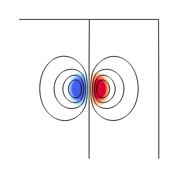
Vorticity distribution and a few streamlines

We now realize that the stream function is not Gallilean invariant. We decide to study the streamlines in the frame that co-moves with the theoretical dipole.

  foreach()
    psi[] += x;
  squares ("omega", map = cool_warm);
  for (double iv = -1; iv <= 1; iv += .25) 
    iso_contour(psi, iv);
  save("result2.png");
}

the resulting file is called result2.png;

Vorticity distribution and a few stream lines in the co-moving frame

It reveals that there exists as closed circular streamline around the two vortex structures. This means that fluid inside this so-called atmosphere will be entrained by the dipole.