periodicdipoles.c

Vortex pair collisions in a doubly periodic domain
- The set-up
- Output

Two dipolar vortices exchange their partners in a head-on collision. Snap shots of the partially dyed fluid taken from C.H. Wong (2015), who studied the behaviour of electromagnetically generated dipoles.

Vortex pair collisions in a doubly periodic domain

Because vortex dynamics are fun, and periodic boundaries have recently been enabled on tree grids we simulate some subsequent collisions of two vortex pairs. It is well known that in the case of a head-on colission, the vortex pairs exchange partners.

The set-up

We aim at a set-up where the evolution should show 4 vortex-pair collisions before the vortices re-group with their original partners and end up at the location where they had started (i.e. the exact solution is periodic in time). However, the emergence of chaos may prevent us from coming close to the exact solution.

#define JACOBI 1 //No break in the symmetry because of the grid traversal
#include "navier-stokes/centered.h"

int maxlevel=9,j;
double k=3.83170597;
double temp= 45;
double ue=0.01;
FILE * fpm;
FILE * fpg;

We define a helper function to initialize a vortex pair according to the Lamb-Chaplygin dipolar vortex model. One may define its centered starting location and wheater it is travelling up or down.

void init_lamb(double sig,double xo,double yo){
  refine(sq(x-xo)+sq(y-yo)<2 && level<=(maxlevel+2));
  scalar r[],s[],psi[],omg[];
  foreach() {
    r[] = pow(pow((x-xo),2)+(pow((y-yo),2)),0.5);
    s[] = (x-xo)/r[];
    omg[] = -sig*((r[]<1)*((-2*j1(k*r[])*s[]/(k*j0(k)))))*sq(k);
  }
  boundary({omg});
  poisson(psi,omg);
  boundary({psi});
  foreach(){
    u.x[] += ((psi[0,1]-psi[0,-1])/(2*Delta));
    u.y[] += -(psi[1,0]-psi[-1,0])/(2*Delta);
  }
}
int main(){
  TOLERANCE=10E-6;
  foreach_dimension() 
    periodic(left); // Yay!
  L0=20.;
  X0=Y0=-L0/2.;

We run for two scenarios, with and without an offset such that the dipoles do not collide on domain boundaries (or vertices).

  for ( j=0;j<2;j++){ 
    run();
  }
}

Initialize the vortices such that they first collide at approximately t=5. We use two different starting locations.

event init(t=0){
  N=1<<(maxlevel-2);
  char name[100];
  sprintf(name,"data%d.data",j);
  fpm = fopen(name,"w");
  sprintf(name,"ppm2mp4 vort%d.mp4",j+1);
  fpg = popen (name, "w");
  double xo1,yo1,yo2;
  if (j == 0){
    xo1=0; yo1=5; yo2=-5;
  }else{
    xo1=5; yo1=3.5; yo2=-7.5;}
  init_lamb(1.,xo1,yo1);
  init_lamb(-1.,xo1,yo2);
  boundary(all);
}

Without putting too much emphasis, adaption is casually combined with the doubly periodic domain.

event adapt(i++)
  adapt_wavelet((scalar *){u},(double []){ue,ue},maxlevel);


#if 0
event tend(t=temp){
  fclose(fpm);
}
#endif

Output

We monitor some time-series statistics regarding the flow’s evolution.

event diag(i=50;i+=50; i < 1000){
  scalar omg[];
  double p=0.;
  double e=0.;
  double ee=0.;
  int n=0;
  foreach(reduction(+:n)) {
    n++;
    omg[]=(u.x[0,1]-u.x[0,-1] - (u.y[1,0]-u.y[-1,0]))/(2*Delta);
  }
  boundary(all);
  foreach(reduction(+:p) reduction(+:e) reduction(+:ee)){
    p+=pow(omg[],2)*Delta*Delta;
    e+=  (u.x[]*u.x[]+u.y[]*u.y[])*sq(Delta);
    ee+=((u.x[]*u.x[]+u.y[]*u.y[])+(sq(u.x[1]-u.x[-1])*Delta)+(sq(u.y[0,1]-u.y[0,-1])*Delta))*sq(Delta);
  }
  fprintf(fpm,"%g\t%g\t%d\t%d\t%g\t%g\t%g\t%g\n",t,dt,i,n,p,perf.t,e,ee);
}

The evolution of the kinetic energy for both cases is plotted below.


set xlabel 'time' font ",15"
set ylabel 'engergy' font ",15"
set size square
set key bottom left
plot 'data0.data' u 1:7 w l lw 3 t 'Collisions on boundaries' ,\
     'data1.data' u 1:7 w l lw 3 t 'Collisions away from boundaries

(script)

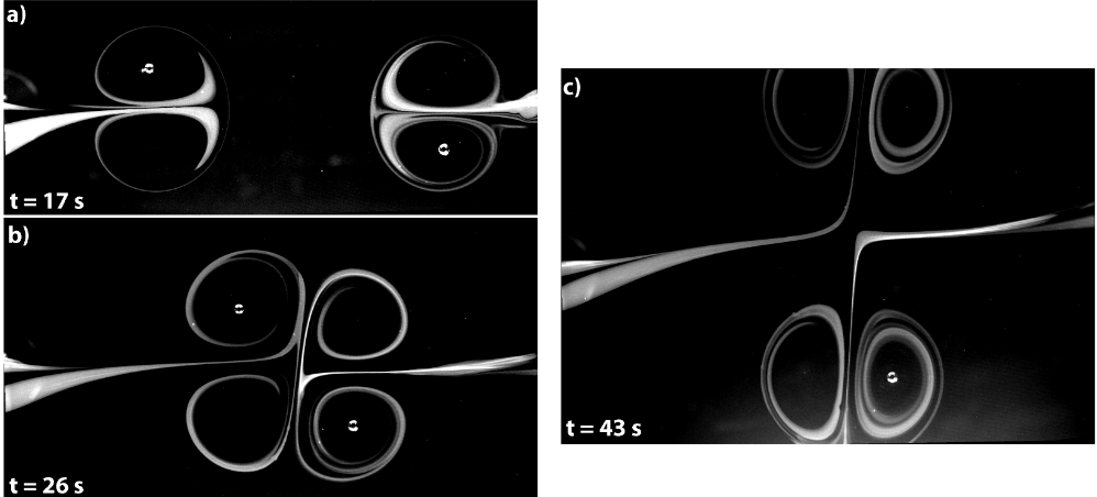
For visual reference we also generate a movie, that will reveal the vortex dynamics by displaying the evolution of the vorticity field.

#if 0
event gfsview(t+=0.2;t<=temp){
  scalar omg[];
  foreach()
    omg[]=(u.x[0,1]-u.x[0,-1] - (u.y[1,0]-u.y[-1,0]))/(2*Delta);
  boundary({omg});
  output_ppm (omg, fpg,n=512,  min = -10, max = 10, linear = true);
}
#endif

I promised it would be fun…

By breaking the symetry of the dipoles, even the smallest numerical errors cause a chaotic evolution of the flow. Hence, numerical errors overwelm the numerically obtained solution and accuracy can then only be expected in a statistical sense.