sandbox/M1EMN/Exemples/bingham_collapse_noSV.c
Collapse of a rectangular visco-plastic heap over a slope
Problem
As a test case we propose the Balmforth collapse of a heap of a 1D non-Newtonian Bingham fluid over a slope S=-Z'_b (S>0). We see the front moving to the right, and the left front going slowly up hill to the left. The flow is of total thickness h. The Y represents the hight at which the stress is equal to the yield stress, hence there is a shear flow of thickness Y; covered by a plug flow of thickness h-Y. Finaly, the flow should stop.
Equations
Using lubrication theory Liu & Mei obtained the flux Q and used conservation of mass, this has been reformulated by Balmforth.
Explicit resolution of \displaystyle \frac{\partial h}{\partial t}+ \frac{\partial Q(h)}{\partial x}=0, \; \text{with} \;\; Q = \frac{Y^2}{6} (3 h - Y) (-Z'_b - \frac{\partial h}{\partial x}) \;\text{and} \;\; Y= \text{max}( h - \frac{B}{|S - \frac{\partial h}{\partial x}|} ,0) this is Balmforth formulation. This formulation is more simple than the Liu & Mei’s one (or Hogg). Note a new formulation by Saramito (to be tested). See Bingham simple example for the derivation.
It can be written for Herschel–Bulkley as well.
The numerical algorithm is very trivial (based on heat equation) and centrered here, it can be inproved (see Fernandez-Nieto et al.).
We added a flux correction to reobtain Huppert second problem in case of large slope S. See a discussion of that in the case of the full Huppert problem which is for B=0, Y=h \displaystyle \frac{\partial h}{\partial t}+ \frac{\partial Q(h)}{\partial x}=0, \; \text{with} \;\; Q = \frac{h^3}{3} (-Z'_b - \frac{\partial h}{\partial x})
Code
mandatory declarations:
#include "grid/cartesian1D.h"
#include "run.h"
definition of the height of interface h, the yield surface Y, its O(\Delta) derivative, ‘hp’ and it O(\Delta^2) derivative hpc, a kind of viscosity \nu, dQ, the divergence of Q, time step, value of the slope, of the Bingham parameter, max time step, increment of time step (for output)
scalar h[];
scalar Y[];
scalar Q[];
scalar hp[],hpc[],nu[],cu[];
scalar dQ[];
double dt,S,B,tmax,inct=0.0001;
char s[80];
Main with definition of parameters
int main() {
  L0 = 2.;
  X0 = -L0/2;
  S = 1.0;
  N = 128;
  DT = (L0/N)*(L0/N)/5 ;
  tmax = 201;
a loop for the three values of Bingham parameter
 for (B = 0.5 ; B <= 2 ; B += 0.75){ //  B = 1.25;  //.5 1.25 2
  sprintf (s, "x-%.2f.txt", B);
  FILE * fp = fopen (s, "w");
  fclose(fp);
  sprintf (s, "shape-%.2f.txt", B);
  FILE * fs = fopen (s, "w");
  fclose(fs);
  inct = DT;
  run();
 }
}
initial elevation: a “rectangular column” of surface 0.5:
print data
//event printdata (t += 1; t <= 100) {
event output (t += inct; t < tmax) {
  double  xf=0,xe=0;
  inct = inct*2;
  inct = min(1,inct);
tracking the front and the end of the heap
  foreach(){
   xf = h[] > 1e-4 ?  max(xf,x) :  xf ;
   xe = h[] > 1e-4 ?  min(xe,x) :  xe ;
  }
save them
  sprintf (s, "front-%.2f.txt", B);
  FILE * f = fopen (s, "w");
  foreach()
    fprintf (f, "%g %g %g \n", fmin((x-xf),0), h[], xe-xf);
  fclose(f);
  fprintf (stderr, "%g %g %g \n", t, xf, xe);
  sprintf (s, "x-%.2f.txt", B);
  FILE * fp = fopen (s, "a");
   fprintf (fp, "%g %g  \n", t, xf);
  fclose(fp);
}
save the hight the flux and the yield surface as a function of time
event printdata (t = {0, 0.0625, 0.25, 1, 4, 100 }  ){
  sprintf (s, "shape-%.2f.txt", B);
  FILE * fp = fopen (s, "a");
  foreach()
    fprintf (fp, "%g %g %g %g %g \n", x, h[], Q[], Y[], t);
  fprintf (fp, "\n");
  fclose(fp);
}
integration
Definition of the flux
double FQ(double h,double Y)
{
  return 1./6*(3*h - Y)*Y*Y ;
  //return (2*(2* pow(h - Y ,2.5) + pow(h,1.5)*(-2*h + 5*Y)))/15.;
  //return (2*( h* pow(h,1.5)))/5.;
  //
}
definition of the derivative of the flux
Y=h- B/|S-\partial_xh| is such that dY/dh is almost 1 \displaystyle c = \frac{d}{dh} (1/6*(3*h - Y(h))*(Y(h))^2) \simeq 1./6*Y*Y* (3 - 1) + 1./3*(3*h - Y)*Y* 1
double FQh(double h,double Y)
{
    return 1./6*Y*Y* (3 - 1) +  1./3*(3*h - Y)*Y* 1;
}


event integration (i++) {
  double dt = DT;
finding the good next time step
dt = dtnext (dt);O(\Delta) down stream derivative
Centered derivative for h' used in the yield criteria for the yield surface Y
Maybe not the best choice…
Yield surface
the flux is taken with the mean value with the next cell, \nu is an intermediate variable, a kind of viscosity (that is why we center)
To avoid oscillations in case of very large slope S the advective part of the flux is corrected with -c (h_i -h_{i-1}), where c=\partial Q_c/\partial h
  foreach()
    cu[] =  S*(FQh(h[-1,0],Y[-1,0]) + FQh(h[0,0],Y[0,0]))/2;
  boundary ({cu});

  foreach()
    Q[] = - nu[] * hp[] + nu[] * S - cu[] * (h[0,0]-h[-1,0]) ;
  boundary ({Q});
derivative O(\Delta) up stream like for heat equation
update h
Run
Then compile and run:
qcc  -g -O2 -DTRASH=1 -Wall bingham_collapse_noSV.c -o bingham_collapse_noSV -lm
./bingham_collapse_noSV > out

make bingham_collapse_noSV.tst;make bingham_collapse_noSV/plots
make bingham_collapse_noSV.c.html
source ../c2html.sh  bingham_collapse_noSV
Results
All this gives h(x,t) and Y(x,t) plotted as a function of x at t={0, 0.0625, 0.25, 1, 4, 100, 400 }
  set term png ;   set output 'cmp.png';
  set ytics font ",8"
  set multiplot layout 3,1 title "collapse of Bingham 1D on a slope"
  set xlabel "x"
  p[-0.4:1.][:1.6]'shape-0.50.txt' t 'B=0.50 h' w l,''u 1:4 t'Y' w l
  p[-0.4:1.][:1.6]'shape-1.25.txt' t 'B=1.25 h' w l,''u 1:4 t'Y'w l
  p[-0.4:1.][:1.6]'shape-2.00.txt' t 'B=2.00 h' w l,''u 1:4 t'Y'w l

  unset multiplot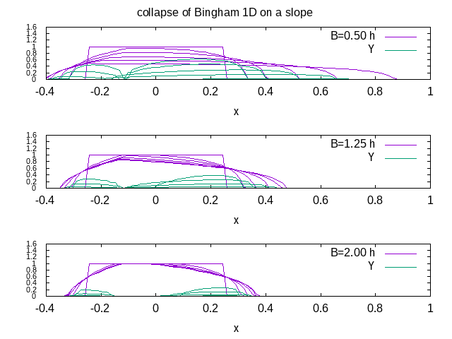
(script)
We now compare with the analytical steady solution of Liu & Mei steady shape. \displaystyle (x -x_{f/e})S = h \pm \frac{B}{S}Log(\frac{B-(\pm S h)}{B}), the front and the end of the final heap compare well
  set term png ;   set output 'std.png';
  set font ",8"
  set multiplot layout 3,1 title "collapse of Bingham 1D on a slope, final shape compared to Liu & Mei "
  set xlabel "x-xf"
  set ylabel "h(x,t)  "
  B=0.5
  p[-1.5:.5][:1]'front-0.50.txt' t 'B=0.50' w l,\
  ''u (($2) + B*log((B-$2)/B) ):2 t'exact' w l,''u (($2)+$3 - B*log((B+$2)/B) ):2 t'exact' w l
  B=1.25
  p[-1.5:.5][:1]'front-1.25.txt' t 'B=1.25' w l,\
  ''u (($2) + B*log((B-$2)/B) ):2 t'exact' w l,''u (($2)+$3 - B*log((B+$2)/B) ):2 t'exact' w l
  B=2.0
  p[-1.5:.5][:1]'front-2.00.txt' t 'B=2.00' w l,\
  ''u (($2) + B*log((B-$2)/B) ):2 t'exact' w l,''u (($2)+$3 - B*log((B+$2)/B) ):2 t'exact' w l
 unset multiplot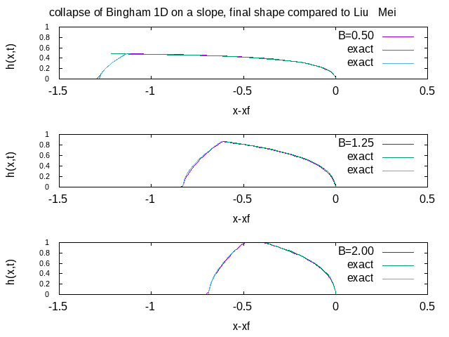
(script)
plot of the front as function of time for the three values of Bingham parameter, the heap is nearly steady at the end…
 set term png ;   set output 'frt.png';
 set xlabel "t"
 set ylabel "xf "
 set logscale x
 p[][:1]'x-0.50.txt' t 'B=0.50' w l,'x-1.25.txt' t 'B=1.25' w l,'x-2.00.txt' t 'B=2.00' w l,.25+sqrt(x)/4
 reset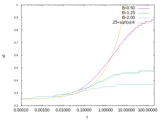
(script)
compare with Balmforth Results
Here the figure extracted from Balmforth 
the results may be improved if we increase the number of points. note that Y has always some imprecision linked to the inverse in its definition.
case B=2reset
set term png ; set output 'B2.png';
X0=218
X1=369
Y0=313
Y1=526.87
unset tics
p[111:370][313:540]'../Img/balmf06.png' binary filetype=png with rgbimage not,\
'shape-2.00.txt' u (X0+($1/(0.49))*(X1-X0)):(($1>-60)?Y0+$2*(Y1-Y0):NaN) t 'h(x,t)' w lp,\
'shape-2.00.txt' u (X0+($1/(0.49))*(X1-X0)):(($1>-60)?Y0+$4*(Y1-Y0):NaN) t 'Y(x,t)' w lp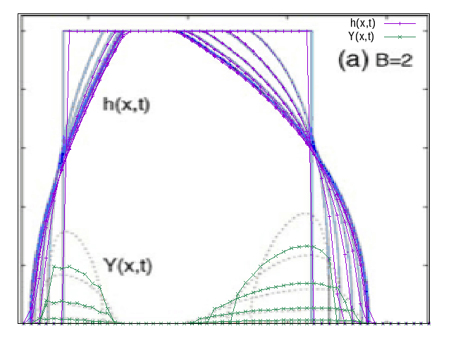
h and Y comparison B=2 (script)
case B=0.5
reset
set term png ;   set output 'Bp5.png';
X0=170
X1=460
Y0=36.53
Y1=249
unset tics
p[37:460][34:262]'../Img/balmf06.png' binary filetype=png with rgbimage not,\
 'shape-0.50.txt' u (X0+($1/(0.90))*(X1-X0)):(($1>-60)?Y0+$2*(Y1-Y0):NaN) t 'h(x,t)' w lp,\
 'shape-0.50.txt' u (X0+($1/(0.90))*(X1-X0)):(($1>-60)?Y0+$4*(Y1-Y0):NaN) t 'Y(x,t)' w lp
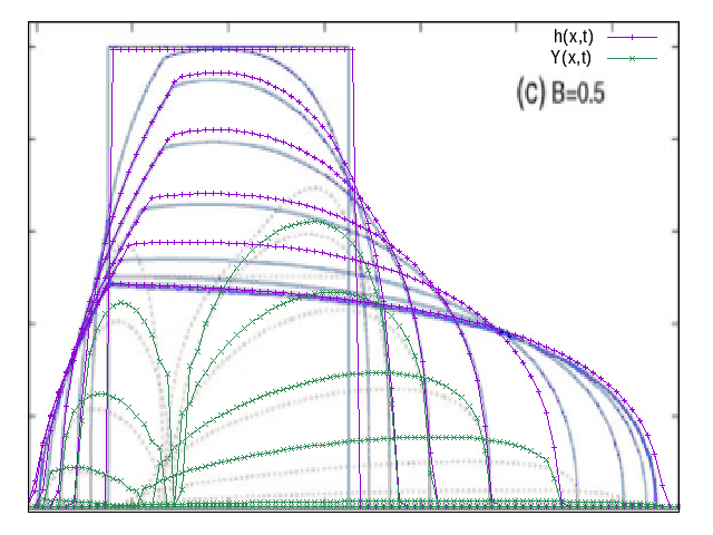
h and Y comparison B=.5 (script)
We notice some small differences, the early collapse seems to be more rapid here than in Balmforth.
case B=1.25
reset
set term png ;   set output 'B1p25.png';
X0=522.4
X1=681
Y0=311.6
Y1=526.87
unset tics
p[406:694][311:538]'../Img/balmf06.png' binary filetype=png with rgbimage not,\
'shape-1.25.txt' u (X0+($1/(0.51))*(X1-X0)):(($1>-60)?Y0+$2*(Y1-Y0):NaN) t 'h' w lp,\
'shape-1.25.txt' u (X0+($1/(0.51))*(X1-X0)):(($1>-60)?Y0+$4*(Y1-Y0):NaN) t 'Y' w lp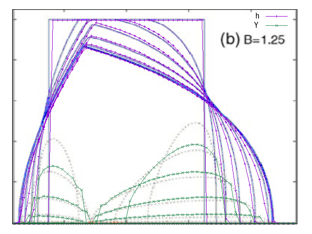
h and Y comparison B=1.25 (script)
idem on original image (for gnuplot pleasure)
 reset
set term png ;   set output 'B1p25bis.png';
 X0=522.4
 X1=681
 Y0=311.6
 Y1=526.87
 unset tics
 p'../Img/balmf06.png' binary filetype=png with rgbimage not,\
 'shape-1.25.txt' u (X0+($1/(0.51))*(X1-X0)):(($1>-60)?Y0+$2*(Y1-Y0):NaN) t 'h' w lp,\
 'shape-1.25.txt' u (X0+($1/(0.51))*(X1-X0)):(($1>-60)?Y0+$4*(Y1-Y0):NaN) t 'Y' w lp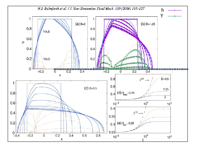
h and Y comparison B=1.25 (script)
Runout as funtion of time compares not so bad
set term png ;   set output 'r.png';
X0=655
X1=810
Y0=132
Y1=310
unset tics
set key center top
plot [475:756][155:290]'../Img/balmf06.png' binary filetype=png with rgbimage not,'x-0.50.txt' u (X0+((log($1))/(10))*(X1-X0)):(((log($1))>-60)?Y0+$2*(Y1-Y0):NaN) w l lw 3 t 'B=0.5','x-1.25.txt' u (X0+((log($1))/(10))*(X1-X0)):(((log($1))>-60)?Y0+$2*(Y1-Y0):NaN) w l lw 3 t 'B=1.25','x-2.00.txt' u (X0+((log($1))/(10))*(X1-X0)):(((log($1))>-60)?Y0+$2*(Y1-Y0):NaN) w l lw 3 t 'B=2'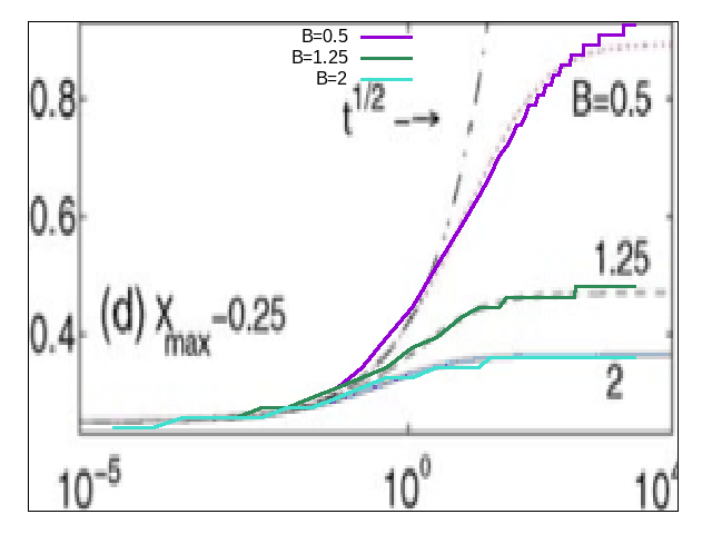
runout as function of B (script)
Links
- Huppert first and secod problems
- Bingham periodic 2D on a slope
- Bingham concrete 2D slump test
- Bingham 1D collapse on a incline
- Herschel-Bulkley 1D collapse on a incline
- Bingham RNSP collapse on a incline
Bibliography
- Neil J. Balmforth, Richard V. Craster, Alison C. Rust, Roberto Sassi “Viscoplastic flow over an inclined surface”, J. Non-Newtonian Fluid Mech. 139 (2006) 103–127
- K.F. Liu, C.C. Mei, “Slow spreading of Bingham fluid on an inclined plane”, J. Fluid Mech. 207 (1989) 505–529.
- H. Huppert “The propagation of two-dimensional and axisymmetric viscous gravity currents over a rigid horizontal surface” JFM vol. 121, p p . 43-58 (1982)
- N. Bernabeu, P. Saramito and C. Smutek, Int. J. Numer. Anal. Model., 11(1):213-228, 2014. “Numerical modeling of shallow non-Newtonian flows: Part II. Viscoplastic fluids and general tridimensional topographies”
- Enrique D. Fernández-Nieto, José M. Gallardo, Paul Vigneaux, “Efficient numerical schemes for viscoplastic avalanches. Part 1: The 1D case” Journal of Computational Physics Volume 264, 1 May 2014, Pages 55–90
Bingham simple example for the derivation.
V1 nov 14 OK Juillet 17 Montpellier, 07/18 Paris