sandbox/M1EMN/Exemples/viscous_collapse_noSV.c
collapse of a rectangular viscous column in 2D
As a simple case we propose the Huppert collapse, this is the explicit resolution of the mass equation for a very viscous flow (viscous stress=pressure gradient) \displaystyle \frac{\partial h}{\partial t}+ \frac{\partial Q(h,\partial_xh)}{\partial x}=0, \text{ with } Q = -\frac{h^3}{3} \frac{\partial h}{\partial x}
Code
mandatory declarations:
#include "grid/cartesian1D.h"
#include "run.h"
definition of the height of interface its O(\Delta) derivative and its O(\Delta^2) derivative, time step
scalar h[];
scalar Q[];
double dt;
Main with definition of parameters
initial elevation: a “double square” of surface 2
print data in stdout
event printdata (t += 10; t <= 500) {
  foreach()
    fprintf (stdout, "%g %g %g %g \n", x, h[], Q[], t);
  fprintf (stdout, "\n");
}
integration
event integration (i++) {
  double dt = DT;
finding the good next time step
dt = dtnext (dt);the flux Q = -\frac{h^3}{3} \frac{\partial h}{\partial x}
  foreach() //_face()
    Q[] = -1./3 * (( h[0,0] - h[-1,0] )/Delta) * pow((h[0,0] + h[-1,0])/2,3);
  boundary ({Q});
update \frac{\partial h}{\partial t}= - \frac{\partial Q(h)}{\partial x}
Run
Then compile and run:
qcc  -g -O2 -DTRASH=1 -Wall viscous_collapse_noSV.c -o viscous_collapse_noSV
./viscous_collapse_noSV > out
To run
make viscous_collapse_noSV.tst
make viscous_collapse_noSV/plots
make viscous_collapse_noSV.c.html

source c2html.sh viscous_collapse_noSV
Results
The analytical solution is obtained in observing that a selfsimilar solution exists \displaystyle h(x,t) = t^{-1/5} (\frac{9}{10} (b^2 - {(xt^{-1/5})}))^{1/3} \text { with } \int_{-b}^{+b} hdx =2. with b^2=\frac{3\ 10^{2/5} \left(\Gamma \left(\frac{2}{3}\right) \Gamma \left(\frac{11}{6}\right)\right)^{6/5}}{\pi ^{9/5}}=1.28338 for mass conservation
In gnuplot type
p[0:2]'out' not w l which gives h(x,t) plotted as a function of x at t=10..500
 set output 'plot1.png'
 set xlabel "x"
 set ylabel "h(x,t)  "
 p[:]'out' not w l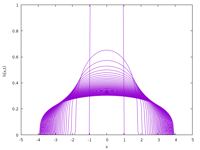
(script)
The self similar solution
p[0:2]'out' u ($1/($4**.2)):($2*($4**.2)),(9./10*(1.28338-x*x))**(1/3.)
which gives h(x,t)t^{1/5} plotted as a function of (xt^{-1/5})
h is zero for (xt^{-1/5}) > b =1.13286
 set output 'plot2.png'
 set xlabel "x/t^{1/5}"
 set ylabel "h(x,t) t^{1/5}"
 p[0:1.5]'out' u ($1/($4**.2)):($2*($4**.2)) t 'num' w l,(9./10*(1.28338-x*x))**(1/3.) t'Self Sim'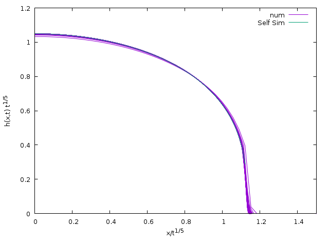
(script)
Links
- http://basilisk.fr/sandbox/M1EMN/Exemples/viscous_collapse.c
- http://basilisk.fr/sandbox/M1EMN/Exemples/viscous_collapse_noSV.c
- http://basilisk.fr/sandbox/M1EMN/Exemples/viscous_collapse_ML.c
Bibliographie
- Huppert “The propagation of two-dimensional and axisymmetric viscous gravity currents over a rigid horizontal surface” JFM 82
- Lagrée M1EMN Master 1 Ecoulements en Milieu Naturel
- Lagrée M2EMN Master 2 Ecoulements en Milieu Naturel
OK v2