sandbox/acastillo/readme

    Andrés’s Sandbox

    I store in this location some of the work done in Basilisk. I work with the Boussinesq equations for natural convection in enclosed cavities but you can also find pieces of code which may be useful in other contexts. More information can be found on this page

    This sandbox is divided in different parts:


    Output fields

    This includes a series of routines to write the resulting fields into several different formats.

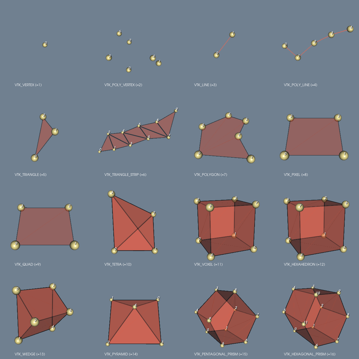
    • output_vtu() - This format is compatible with the VTK XML file format for unstructured grids File formats for VTK version 4.2 which can be read using Paraview. Here, the results are written in plain ASCII. The unstructured grid is required to write results from quadtrees and octrees. Other routines, specific to regular Cartesian grids are also available inside output_fields/ but are not recommended unless storage space is a concern. If used in MPI, each MPI task writes its own file, which may be linked together using a *.pvtu file. An example is available here.

    • in-situ visualisation with catalyst Catalyst is an API specification developed for simulations (and other scientific data producers) to analyze and visualize data in situ. This requires a ParaView release with an implementation of the Catalyst API. This way, we can execute python/paraview scripts while the simulation is running. Works on MPI. Linking is automatic but requires the environment variables CATALYST_INCDIR and CATALYST_LIBDIR , which are usually set when you load the module paraview on a computer cluster. An example is available here. For testing try: sudo apt install paraview paraview-dev export CATALYST_INCDIR=/usr/include/paraview-5.10/catalyst export CATALYST_LIBDIR=/usr/lib/x86_64-linux-gnu/ CC='mpicc -D_MPI=8 -DUSE_CATALYST ' make test_output5.tst cd test_output5 mpirun -n 8 ./test_output5 ../sample_scripts/live_visu.py

    • output_xmf() This routine is compatible with the XDMF Model and Format which can be read using Paraview or Visit. Data is split in two categories: Light data and Heavy data. Light data is stored using eXtensible Markup Language (XML) to describe the data model and the data format. Heavy data is composed of large datasets stored using the Hierarchical Data Format HDF5. As the name implies, data is organized following a hierarchical structure. HDF5 files can be read without any prior knowledge of the stored data. The list of software capable of reading HDF5 files includes Visit, Paraview, Matlab, and Tecplot, to name a few. The type, rank, dimension and other properties of each array are stored inside the file in the form of meta-data. Additional features include support for a large number of objects, file compression, a parallel I/O implementation through the MPI-IO or MPI POSIX drivers. Using this format requires the HDF5 library, which is usually installed in most computing centers or may be installed locally through a repository. Linking is automatic but requires the environment variables HDF5_INCDIR and HDF5_LIBDIR, which are usually set when you load the module hdf5. An example is available here.

    • For testing the XDMF format try:

    
      sudo apt install libhdf5-dev hdf5-helpers  hdf5-tools
      export HDF5_INCDIR=/usr/include/hdf5/serial
      export HDF5_LIBDIR=/usr/lib/x86_64-linux-gnu/hdf5/serial
      make test_output4.tst
    • For testing using MPI try:
    
      sudo apt install libhdf5-mpi-dev hdf5-helpers  hdf5-tools
      export HDF5_INCDIR=/usr/include/hdf5/openmpi
      export HDF5_LIBDIR=/usr/lib/x86_64-linux-gnu/hdf5/openmpi
      CC='mpicc -D_MPI=4' make test_output4.tst
    • After the simulation, it is possible inspect the contents of the Heavy data from the terminal using:
    
    >> h5ls -r fields.h5
    /                        Group
    /000000                  Group
    /000000/Cell             Group
    /000000/Cell/T           Dataset {512, 1}
    /000000/Cell/pid         Dataset {512, 1}
    /000000/Cell/u.x         Dataset {512, 3}
    /000000/Geometry         Group
    /000000/Geometry/Points  Dataset {900, 3}
    /000000/Topology         Dataset {512, 8}
    ...
    

    Input fields

    This includes a series of routines to read existing results and use them as initial conditions for a new simulation.

    • input_matrix() - This format reads a binary file written using output_matrix() or output_matrix_mpi() and loads it into a field selected by the user. For instance, to read a square field of size L0 defined inside a regular Cartesian grid with N points, starting from (X0,Y0) stored in a file “example.bin” and load it into a scalar field,
        scalar T[];
        ...
        fprintf (stderr, "Reprising run from existing initial conditions ... \n");
        fprintf (stderr, "Read from example.bin ... \n");
    
        FILE * fp = fopen("example.bin", "r");
        if (!fp) printf("Binary file not found");
        input_matrix(T,fp,N,X0,Y0,L0);
        fclose (fp);
        ...
        boundary(T);

    An example on how to generate some arbitrary initial condition using matlab is available here


    Boussinesq equations

    This includes an implementation of the Boussinesq equations by combining the centered Navier-Stokes solver (see centered.h) and an advection-diffusion problem for the temperature field using the diffusion solver (see diffusion.h) and the advection of a passive scalar.

    For this work, we focus on the Rayleigh-Bénard convection which involves a horizontal fluid layer of height H, which is heated uniformly from below and cooled uniformly from above in the presence of gravity. By convention the gravity force \vec{g}=(0, −g, 0) is opposed to the unit vector in the y-direction. \displaystyle T = T_{bot} \quad\quad \text{ at } y=0 \displaystyle T = T_{top} = T_{bot} - \Delta T \quad\quad \text{ at } y=H Ideally the fluid layer extends over an infinite plane, but in practice, one must also consider the fluid container, usually a cylinder or a square box.

    The Boussinesq approximation states that density changes in the fluid are neglected except in the buoyance term. Additionally, we assume the density to depend linearly on the temperature only, \displaystyle \rho(T) = \rho_{ref}(1-\beta(T-T_ {ref})) where \beta is the coefficient of thermal expansion at the reference state (T_{ref},p_{ref}). In our case, the reference temperature is taken as T_{ref}=(T_{top}+T_{bot})/2.

    By introducing this approximation into the Navier-Stokes equation, we obtain the following Boussinesq system : \displaystyle \nabla \cdot \vec{u} = 0 \displaystyle \partial_t \vec{u} + \nabla \cdot \left(\vec{u} \otimes \vec{u} \right) = -\frac{1}{\rho_{ref}}\nabla p^* + \nabla \cdot \left( \nu_{ref} \nabla \vec{u} \right) - \beta(T-T_{ref}) \vec{g} \displaystyle \partial_t T + \nabla \cdot \left( \vec{u} T \right) = \nabla \cdot \left( \kappa_{ref} \nabla T \right) + S_q Since fluid properties are always evaluated at the reference state, in the following we drop the subscript everywhere except for the reference temperature T_{ref}.

    Dimensionless Parameters

    We define the characteristic mass [M], length [L], temperature [Θ], and velocity [U] scales as follows. The relevant length scale corresponds to the height of the fluid layer H, while the temperature scale is fixed by the temperature difference \Delta T between the top and bottom plates. A characteristic velocity scale corresponds to the free-fall velocity divided by Pr^{0.5} \displaystyle [M] = \rho H^3 \quad\quad [L] = H \quad\quad [\Theta] = \Delta T \quad\quad [U] = \frac{k}{H}\sqrt{\frac{g\beta\Delta T H^3}{\kappa\nu}} We proceed to define a set of non-dimensional variables. From this point on, quantities are written in dimensionless form only.

    Dimensionless Boussinesq equations

    The Oberbeck-Boussinesq equations may be written in dimensionless form as \displaystyle \nabla \cdot \vec{u} = 0 \displaystyle \partial_t \vec{u} + \nabla \cdot \left(\vec{u} \otimes \vec{u} \right) = -\nabla p + \nabla \cdot \left( PrRa^{0.5} \nabla \vec{u} \right) + Pr\theta\vec{e}_y \displaystyle \partial_t \theta + \nabla \cdot \left( \vec{u} \theta \right) = \nabla \cdot \left( Ra^{-0.5} \nabla \theta \right) which is fully defined by two dimensionless numbers, the Rayleigh and Prandtl numbers \displaystyle Ra \equiv \frac{g H \beta (T_{bot}-T_{top})}{\kappa\nu} \quad\quad\quad Pr \equiv \frac{\nu}{\kappa}

    In addition to the relevant boundary and initial conditions.

    Numerical method (2nd order global accuracy)

    The formulation of the Boussinesq equations uses the fractional-step method using a staggered in time discretization of the velocity and the scalar fields: one supposes the velocity field to be known at time n and the scalar fields (pressure, temperature, density) to be known at time n−1/2, and one computes velocity at time n+1 and scalars at time n+1/2. We use a pressure correction scheme for the velocity-pressure coupling. In this scheme, the pressure term is treated explicitly to obtain a provisional velocity field \vec{u}^∗ which may not be divergence-free. A correction term is obtained by projecting the provisional velocity into a divergence-free space.

    The (temporal) discretization of the Boussinesq equations would have the following form:

    1. A Helmholtz problem for the temperature field \displaystyle \frac{\theta^{n+1/2}-\theta^{n-1/2}}{\Delta t} + \nabla \cdot \left( \vec{u}^n \theta^n \right) = \nabla \cdot \left( Ra^{-0.5} \nabla \theta^{n+1/2} \right)
    2. A Helmholtz problem for the provisional velocity field \displaystyle \frac{\vec{u}^*-\vec{u}^n}{\Delta t} + \nabla \cdot \left(\vec{u}^{n+1/2} \otimes \vec{u}^{n+1/2} \right) = PrRa^{0.5} \frac{1}{2} \nabla \cdot \left( \nabla \vec{u}^* + \nabla \vec{u}^n \right) + Pr\theta^{n+1/2}\vec{e}_y
    3. A Poisson problem for the pressure field \displaystyle \nabla^2 p^{n+1/2} = -\frac{1}{\Delta t}\nabla\cdot\vec{u}^{*}
    4. and a correction to the velocity field. \displaystyle \vec{u}^{n+1} = \vec{u}^{*} - \Delta t \nabla p^{n+1/2}

    Here the velocity advection term \nabla \cdot \left(\vec{u}^{n+1/2} \otimes \vec{u}^{n+1/2} \right) and the temperature advection term \nabla \cdot \left( \vec{u}^n \theta^n \right) are estimated by means of the Bell–Colella–Glaz second-order unsplit upwind scheme. Each step is divided into several sub-steps, each associated to a particular event.

    Working examples

    Instead of writing an entirely new code, existing blocks of code were combined to solve Boussinesq equations. A series of working examples are available below: