sandbox/easystab/KH_temporal_viscous.m
This document belongs to the easystab project, please consult the main page of the project for explanations.
The present program was specifically designed as a support for the course “Introductions to hydrodynamical instabilities” for the “DET” Master’s cursus in Toulouse. For the underlying theory please see Lecture notes for chapter 7
To use this program: click “raw page source” in the left column, copy-paste in the Matlab/Octave editor, and run.
Kelvin-Helmholtz instability of a shear layer
(temporal analysis, viscous case, uvp formulation)
(This code is adapted from sandbox/easystab/kelvin_helmholtz_hermite.m from the easystab project).
We start from the linearised Navier-Stokes equations around a parallel base flow defined as U(y). We look for solutions under eigenmode form : \displaystyle [u,v,p] = [\hat u(y), \hat v(y), \hat p(y)] e^{i k x} e^{-i \omega t}
According to the lecture notes, the problem can be set in matricial form as follows:
\displaystyle - i \omega {\mathcal B} \, \hat{q} = {\mathcal A} \, \hat{q}
where \hat{q} = [\hat u(y), \hat v(y), \hat p(y)]. The building of the matrices and resolution of the eigenvalue problem is done in the function KH defined at the end of this document.
function [] = main()
close all;
global y D DD w Z I U Uy discretization

% physical parameters
alpha=0.5;    % the wave number
Re=20;    % the Reynolds number

% numerical parameters
N=100;      % the number of grid points
loopk = 1; % set to 0 to skipp the loops over k and Re to build the curves
Derivation matrices
Here we use Chebyshev discretization with stretching. See differential_equation_infinitedomain.m to see how this works.
discretization = 'chebInfAlg'; %
[D,DD,w,y] = dif1D(discretization,0,3,N,0.99999);

Z=zeros(N,N); I=eye(N);
Ndim=N;

% base flow
U=tanh(y);
Uy=(1-tanh(y).^2);
We compute the eigenvalues/eigenmodes with the function KH, defined at the end of this program
[s,UU] = KH(alpha,Re,N);
omega = 1i*s;
Plotting the spectrum
figure(1);
for ind=1:length(s)
  h=plot(real(omega(ind)),imag(omega(ind)),'*'); hold on
  set(h,'buttondownfcn',{@plotmode,UU(:,ind),omega(ind),alpha});
end
xlabel('\omega_r');
ylabel('\omega_i');
ylim([-1 .25]);
xlim([-.75 .75]);
title({['Temporal spectrum for k = ',num2str(alpha), ', Re = ',num2str(Re)], 'Click on eigenvalues to see the eigenmodes'});
set(gcf,'paperpositionmode','auto');
print('-dpng','-r80','KH_temporal_viscous_spectrum.png');
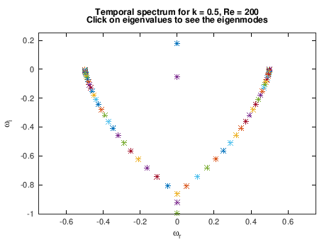
** Figure : Temporal spectrum of a tanh shear layer
plotmode([],[],UU(:,1),omega(1),alpha);

pause(0.1);
set(gcf,'paperpositionmode','auto');
print('-dpng','-r80','KH_temporal_viscous_mode.png');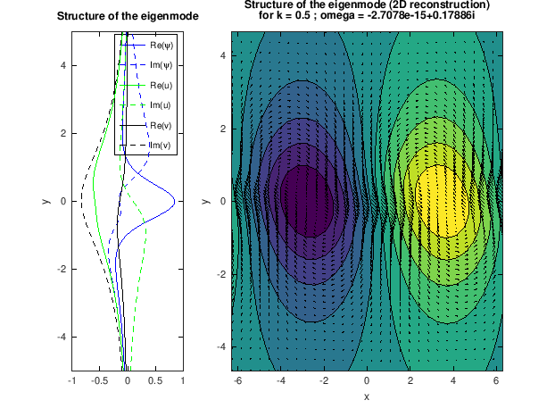
** Figure : Unstable eigenmmode of the tanh shear layer for k=0.5
Now we do loops over k and Re to plot the growth rate curves
\omega_i(k)
%%
if loopk
  for Re = [3 10 30 100 300 1000]
    alphatab = 0:.01:1.2;
    lambdatab = [];
    for alpha=alphatab
        [s,UU] = KH(alpha,Re,N);
        lambdatab = [lambdatab s(1)];
    end
    figure(3);hold on;
    plot(alphatab(1:length(lambdatab)),real(lambdatab));hold on;
    hold on;
    pause(0.1);
  end

 figure(3);
    legend('Re=3','Re=10','Re=30','Re=100','Re=300','Re=1000');
    legend('Location','South');
    xlabel('k');ylabel('\omega_i');
    title('growth rate for several values of Re');

    set(gcf,'paperpositionmode','auto');
    print('-dpng','-r80','KH_temporal_viscous_curves.png');

end
%%
end
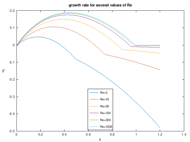
** Figure : results for the Kelvin-Helmholtz instability (temporal) of a tanh shear layer
Function KH
%%
function [s,UU] = KH(alpha,Re,N)
global y D DD w Z I U Uy discretization % to use these objects within the function

% renaming the differentiation matrices
dy=D; dyy=DD;
dx=1i*alpha*I; dxx=-alpha^2*I;
Delta=dxx+dyy;
Theory
The problem is as follows:
\displaystyle - i \omega {\mathcal B} \, \hat{q} = {\mathcal A} \, \hat{q}
with \displaystyle {\mathcal B} = \left[ \begin{array}{ccc} 1 & 0 & 0 \\ 0 & 1 & 0 \\ 0 & 0 & 0 \end{array} \right]
\displaystyle {\mathcal A} = \left[ \begin{array}{ccc} -i k \bar{U} + Re^{-1} ( \partial_y^2 - k^2) & - \partial_y \bar{U} & - i k \\ 0 & -i k \bar{U} + Re^{-1} ( \partial_y^2 - k^2) & - \partial_y \\ i k & \partial_y & 0 \end{array} \right]
For the underlying theory please see Lecture notes for chapter 7*
System matrices
% the matrices
S=-diag(U)*dx+Delta/Re;
A=[ ...
    S, -diag(Uy), -dx; ...
    Z, S, -dy; ...
    dx, dy, Z];
E=blkdiag(I,I,Z);

% Boundary conditions
if(strcmp(discretization,'her')==1)
    indBC = [];
    % No boundary conditions are required with Hermite interpolation which
    % naturally assumes that the function tends to 0 far away.
else
    % Dirichlet conditions are used for fd, cheb, etc...
    III=eye(3*N);
    indBC=[1,N,N+1,2*N];
    C=III(indBC,:);
    A(indBC,:)=C;
    E(indBC,:)=0;
end

% computing eigenmodes

[UU,S]=eig(A,E);

% sort the eigenvalues by decreasing real part and remove the spurious ones
s=diag(S);  [t,o]=sort(-real(s)); s=s(o); UU=UU(:,o);
rem=abs(s)>1000; s(rem)=[]; UU(:,rem)=[];

end %function KH
Function plotmode
function [] = plotmode(~,~,mode,omega,alpha)
    global y dy dyy
    Yrange = 5;
    figure(2);hold off;
    N = length(y);
    u = mode(1:N);
    v = mode(N+1:2*N);
    p = mode(2*N+1:3*N);
    %vorticity = (dy*u)-1i*k*v;
    subplot(1,3,1);hold off;
    plot(real(u),y,'b-',imag(u),y,'b--');hold on;
    plot(real(v),y,'g-',imag(v),y,'g--');hold on;
    plot(real(p),y,'k-',imag(p),y,'k--');hold on;
    ylabel('y'); ylim([-Yrange,Yrange]);
%legend({'$Re(\hat u)$','$Im(\hat u)$','$Re(\hat v)$','$Im(\hat v)$','$Re(\hat p)$','$Im(\hat p)$'},'Interpreter','latex')
    legend({'Re(\psi)','Im(\psi)','Re(u)','Im(u)','Re(v)','Im(v)'});
    title('Structure of the eigenmode');
    % plot 2D reconstruction
    Lx=2*pi/alpha; Nx =30;  x=linspace(-Lx/2,Lx/2,Nx);
    p(abs(y)>Yrange,:)=[];
    u(abs(y)>Yrange,:)=[];
    v(abs(y)>Yrange,:)=[];
    %vorticity(abs(y)>Yrange,:)=[];
    yy = y;
    yy(abs(y)>Yrange)=[];
    pp = 2*real(p*exp(1i*alpha*x));
    uu=2*real(u*exp(1i*alpha*x));
    vv=2*real(v*exp(1i*alpha*x));
    %vorticityvorticity=2*real(vorticity*exp(1i*alpha*x));
    subplot(1,3,2:3); hold off;
    contourf(x,yy,pp,10); hold on;
    quiver(x,yy,uu,vv,'k'); hold on;
    %axis equal;
    xlabel('x'); ylabel('y'); title({'Structure of the eigenmode (2D reconstruction)',['for k = ',num2str(alpha) , ' ; omega = ',num2str(omega)]});
end% function plotmode
Exercices/Contributions
- Please compare the results with the inviscid ones obtained using the program KH_temporal_inviscid.m
- Please validate the results by comparing with the litterature (Drazin & Reid)
- Please try other discretisation methods, for instance Hermite —-> sandbox/easystab/kelvin_helmholtz_hermite.m
- Please look at the structure of the adjoint eigenmode and compute the nonnormality factor.
%}