sandbox/easystab/david/KH_temporal_inviscid.m
Kelvin-Helmholtz instability of a shear layer
(temporal analysis, viscous case, Rayleigh Equation)
We study the stability of a parallel shear flow U(y) in the inviscid case. We solve the Rayleigh equation, written as follows :
\displaystyle (U - c) \Delta \hat \psi + U_{yy} \hat \psi = 0
function [] = main()
clear all; close all;
global y dy dyy w Z I U Uy Uyy
loopk = 1; % set to 0 to skipp the loop over k
Derivation matrices
Here we wish to solve a problem in an infinite domain. We use Chebyshev discretization with stretching. See differential_equation_infinitedomain.m to see how this works.
N=51;      % the number of grid points
discretization = 'chebInfAlg';
[dy,dyy,w,y] = dif1D(discretization,0,3,N,0.9999);
Z=zeros(N,N); I=eye(N);
Base flow
The base flow is U(y) = tanh(y).
We also need to compute its first and second derivatives:
U=tanh(y);
Uy=(1-tanh(y).^2);
Uyy = -2*tanh(y).*(1-tanh(y).^2);
Eigenvalue computation
We compute the eigenvalues/eigenmodes with the function KH_inviscid, defined at the end of this program.
alpha=0.5;    % the wave number

[c,UU] = KH_inviscid(alpha,N);
omega = c*alpha;
Plot the spectrum :
figure(1);
for ind=1:length(omega)
  %%%% plot one eigenvalue
  h=plot(real(omega(ind)),imag(omega(ind)),'*'); hold on
  %%%%  assign the corresponding event on click
  set(h,'buttondownfcn',{@clickmode,UU(:,ind),omega(ind),y});
end

xlabel('\omega_r');
ylabel('\omega_i');
title({['Temporal spectrum for k = ',num2str(alpha)], 'Click on eigenvalues to see the eigenmodes'});

 set(gcf,'paperpositionmode','auto');
 print('-dpng','-r80','KH_temporal_inviscid_spectrum.png');
** Figure : Temporal spectrum of a tanh shear layer
Plot the unstable eigenmode :
psiM = UU(:,1);
psiM = psiM/psiM(round((N+1)/2));%normalisation
figure(2);
subplot(1,3,1);
plot(real(psiM),y,'r-',imag(psiM),y,'r--');
ylabel('y'); ylim([-5,5]);
legend({'$Re(\hat \psi)$','$Im(\hat \psi)$'},'Interpreter','latex')
title('Structure of the eigenmode');

Lx=2*pi/alpha; Nx =30;  x=linspace(-Lx/2,Lx/2,Nx);
psipsi = 2*real(psiM*exp(1i*alpha*x));
uu=2*real(dy*psiM*exp(1i*alpha*x));
vv=2*real(-1i*alpha*psiM*exp(1i*alpha*x));
sely=1:2:N;
subplot(1,3,2:3);
quiver(x,y(sely),uu(sely,:),vv(sely,:),0.2,'k'); hold on
surf(x,y,psipsi,'facealpha',0.5); shading interp;
axis([x(1),x(end),y(1),y(end)]);
xlabel('x'); ylabel('y'); title('Structure of the eigenmode (2D reconstruction)');
ylim([- 5 5]);
pause(0.1);
set(gcf,'paperpositionmode','auto');
print('-dpng','-r80','KH_temporal_inviscid_mode.png');

** Figure : Unstable eigenmmode of the tanh shear layer for k=0.5
Loop over k to draw the amplification rate as function of the wavenumber
if loopk
    alphatab = 0:.01:1.;
    lambdatab = [];
    for alpha=alphatab
        [s,~] = KH_inviscid(alpha,N);
        lambdatab = [lambdatab alpha*s(1)];
        figure(4);
        plot(alphatab(1:length(lambdatab)),imag(lambdatab),'b');hold on;
        pause(0.1);
    end
    ylabel('\omega_i');
    xlabel('k');
    title('Growth rate as function of k');
    set(gcf,'paperpositionmode','auto');
    print('-dpng','-r80','KH_temporal_inviscid.png');

end%if loopk

end%function main
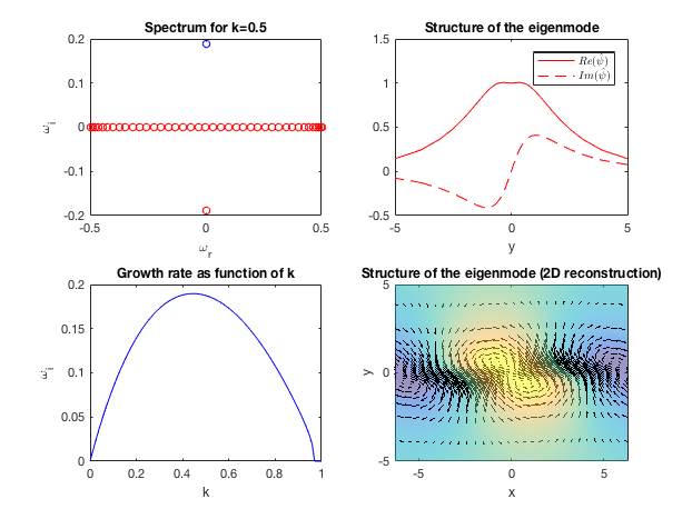
** Figure : results for the Kelvin-Helmholtz instability (temporal) of a tanh shear layer
Function KH_inviscid
Here is the function to compute the eigenvalues/eigenmodes.
function [s,UU] = KH_inviscid(alpha,N)

global y dy dyy I U Uyy

%differential operators
dx=1i*alpha*I; dxx=-alpha^2*I;
Delta=dxx+dyy;

% the matrices
B=Delta;
A=diag(U)*Delta-diag(Uyy);

%Boundary conditions : we use Dirichlet at the boundaries of the stretched domain
indBC=[1,N];
A(indBC,:)=I(indBC,:);
B(indBC,:)=0;

% compute the eigenmodes
[UU,S]=eig(A,B);

% sort the eigenvalues by increasing imaginary part
s=diag(S);  [~,o]=sort(-imag(s)); s=s(o); UU=UU(:,o);
rem=abs(s)>1000; s(rem)=[]; UU(:,rem)=[];

end%function KH_inviscid

function [] = clickmode(~,~,psiM,omega,y)
    figure(10);
    psiM = psiM/psiM(round((length(psiM)+1)/2));
    plot(real(psiM),y,'b',imag(psiM),y,'b--');
    title([' Eigenmode structure for \omega = ',num2str(omega)]);
    legend('\psi_r','\psi_i');
    ylabel('y');
    ylim([-10,10]);
end% function clickmode
Exercices/Contributions
- Please check the convergence of the results by comparing with other discretization methods (e.g. Hermite)
- Please modify the program to treat the case of a 2D jet defined as U(y) = 1/cosh(y)^N where N is an integer defining the ‘steepness’ of the profile (try for instance N=1 for a smooth profile and N=10 for a very steep profile). Compare the latter case with theoretical results for a “top-hat” jet. You may need to adapt the mesh parameters to have enough points in the region of the steep gradients !
%}