sandbox/easystab/diffmat_mapping.m
Differentiation matrices for a non-rectangular domain in 2D
Please see diffmat_mapping_map2D.m for the same code but using the function map2D.m.
The differentiation matrices are at the core of the codes showed here. Until now we have used rectangular domains. We can make the method much more useful and general if we can change the shape of the domain. We show here a straghtforward method based on the mapping of the computational rectangular mesh into something else. This is all based on the formula for composed derivatives. If we call \tilde{x} and \tilde{y} the original computational space variables and we map them into x and y the physical space variables. Then if we have a function f on this physical domain and we want to compute its (physical space) derivatives, then we do \displaystyle
\frac{\partial f}{\partial x}=\frac{\partial f}{\partial \tilde{x}} \frac{\partial \tilde{x}}{\partial x}
and \displaystyle
\frac{\partial f}{\partial y}=\frac{\partial f}{\partial \tilde{y}} \frac{\partial \tilde{y}}{\partial x}.
Based on this, we see that if we can compute the computational derivative \displaystyle
\frac{\partial f}{\partial \tilde{x}},
we just need to multiply (rescale) the result with a derivative of the mapping
\displaystyle
\frac{\partial \tilde{x}}{\partial x},
Thus building the physical space differentiation matrices ammounts to computing first the rescaling coefficients. The formula is quick and simple for the first derivatives, and a little longer for the second derivatives.
In this code, we first build the 2D differentiation for the rectangular domain, then map it and build the associated differentiation matrices.
clear all; clf

% parameters and flags
Nx=21; % gridpoints in x
Ny=22; % gridpoints in x
Lx=pi; % domain size in x
Ly=pi; % domain size in y

% 1D and 2D differentiation matrices
[d.x,d.xx,d.wx,x]=dif1D('cheb',0,Lx,Nx,3);
[d.y,d.yy,d.wy,y]=dif1D('cheb',0,Ly,Ny,3);
[D,l,X,Y,Z,I,NN]=dif2D(d,x,y);
The mapping
Coded as it is here is very general, since we decided to use the numerical derivatives of the mapping. We could have decided to use an analytical mapping, then derived all the coefficients by hand and put them one by one in the code (this is what we do in free_surface_navier_stokes.m). Instead, you just do here the transformations that you like on the computational grid: stretch, compress, distort… then all the coefficients are computed using the numerical differentiation matrices.
For this example, we strech in y increasingly as x grows with a linear law, and stretch in x with a cosine. The actual mapping here is described by etay and etax. The visual aspect of the mapped domain is shown in a figure below.
% mapping of the grid
etay=1+0.1*x;
etax=1-0.1*cos(y);
X=X.*repmat(etax,1,Nx);
Y=Y.*repmat(etay',Ny,1);

% Derivatives of the mapping
xx=D.x*X(:); xy=D.y*X(:);   yx=D.x*Y(:);  yy=D.y*Y(:);
yyy=D.yy*Y(:);   xxx=D.xx*X(:);   yxy=D.y*yx;  yxx=D.xx*Y(:);   xyy=D.yy*X(:);   xyx=D.x*xy;
jac=xx.*yy-xy.*yx;

% diff matrices
D.Mx=diag(yy./jac)*D.x-diag(yx./jac)*D.y;
D.My=-diag(xy./jac)*D.x+diag(xx./jac)*D.y;

D.Mxx=diag((yy./jac).^2)*D.xx ...
     +diag((yx./jac).^2)*D.yy ...
     +diag((yy.^2.*yxx-2*yx.*yy.*yxy+yx.^2.*yyy)./jac.^3)*(diag(xy)*D.x-diag(xx)*D.y) ...
     +diag((yy.^2.*xxx-2*yx.*yy.*xyx+yx.^2.*xyy)./jac.^3)*(diag(yx)*D.y-diag(yy)*D.x);
D.Mxx2=-2*diag(yx.*yy./jac.^2)*(D.y*D.x);

D.Myy=diag((xy./jac).^2)*D.xx ...
     +diag((xx./jac).^2)*D.yy ...
     +diag((xy.^2.*yxx-2*xx.*xy.*yxy+xx.^2.*yyy)./jac.^3)*(diag(xy)*D.x-diag(xx)*D.y) ...
     +diag((xy.^2.*xxx-2*xx.*xy.*xyx+xx.^2.*xyy)./jac.^3)*(diag(yx)*D.y-diag(yy)*D.x);
D.Myy2=-2*diag(xx.*xy./jac.^2)*(D.y*D.x);

% the differentiation matrices
D.x=D.Mx; D.xx=D.Mxx+D.Mxx2;
D.y=D.My; D.yy=D.Myy+D.Myy2;
Showing the matrices and the mesh
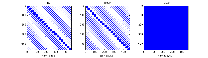
In the above lines of code, we have built the second derivatives in two parts: the part that have cross derivatives (D.M??2) wich contain multiplications of differentiation in two different directions D.x*D.y, and the one that have not. This is usefull for systems with many degrees of freedom, because the cross-derivative are full matrices. For large systems, it is good to have banded differentiation matrices, like for instance obtained from finite difference, and keep this structure using a sparse format for storing the matrices in memory.
% showing the structure of the matrices
figure(1)
subplot(1,3,1); spy(D.x); title('D.x')
subplot(1,3,2); spy(D.Mxx); title('D.Mxx')
subplot(1,3,3); spy(D.Mxx2); title('D.Mxx2')
The mesh and the structure of the matrices
%%%% test the mapping
f=cos(X).*sin(Y);
fx=-sin(X).*sin(Y); fxx=-cos(X).*sin(Y);
fy=cos(X).*cos(Y);  fyy=-cos(X).*sin(Y);

figure(2)
subplot(1,3,1); mesh(X,Y,0*X); view(2); xlabel('x'); ylabel('y'); title('the mapped mesh')
subplot(1,3,2); mesh(X,Y,fx);  xlabel('x'); ylabel('y'); title('analytical derivative in x')
subplot(1,3,3); mesh(X,Y,reshape(D.x*f(:),Ny,Nx));  xlabel('x'); ylabel('y'); title('numerical derivative in x');
Result
The figure below shows the shape of the mapped physical domain, and the visual aspect of the x derivative, both analytical and numerical.
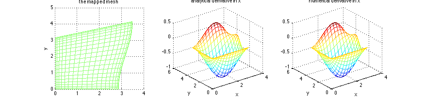
Comparison of analytical and numerical derivatives
% quantifying the error
ex=norm(fx(:)-D.x*f(:))
ey=norm(fy(:)-D.y*f(:))
exx=norm(fxx(:)-D.xx*f(:))
eyy=norm(fyy(:)-D.yy*f(:))
Size of the approximation error
The last commands give this screen output, approximation error close to machine accuracy.
- ex = 4.2286e-11
- ey = 2.6175e-10
- exx = 8.6893e-10
- eyy = 1.8709e-08
Links
The operations on the differentiation matrices for the mapping that we explain and test here are embeded in the function map2D.m, please use this function when you write your own codes. See diffmat_mapping_map2D.m for the same code as here but using map2D.m instead of doing explicitely all the operations.
To test the mapping on a differential equations, please see poisson_2D_mapping.m, where we solve a Poisson problem on a stretched mesh.
The streching that we show here is used in venturi.m for the flow in a pipe with a local neck that induces a flow separation.
A mapping similar to here is used in peristalsis.m, but in that code the differentiation matrices assume periodicity in the x direction so we need to take care of that when computing numerically the derivative of the mapping.
Another way to have more general shapes of meshes is to patch together several rectangular domains. This is shown in multi_domain_2D.m and multi_domain_2D_tri.m. In poisson_2D_hollow_disc.m we combine mesh mapping and mesh patching.
Exercices/Contributions
- Please do a convergence study with the grid
- Please try another deformation of the grid and do the testing (you can deform it very much and see how the accuracy degrades)
- Please do the same as here but using finite difference for the differentiation matrices