sandbox/easystab/meniscus_overturn.m
Overturning meniscus
This code, just as for meniscus.m, comptes the shape of a meniscus using the Newton iteration. The difference is that here we use a method that allows overturning of the fluid interface. This will be useful when drawing the bifurcation diagram for this nonlinear system, because there is a fold in the bifurcation diagram after which the meniscus shape is overturning and unstable.
For this we use an arclength parameterization of the interface with parameter s going from 0 at the wall to 1 at the right end of the domain. The interface is described by \displaystyle x(s), y(s), \theta(s) the horizontal and vertical position at arclength s and \theta is the angle between the interface and the horizontal. note here that we could describe an overturning interface just with x and y but using as well \theta will give simpler equations and simpler jacobian. Looking at an element of length of the interface we find \displaystyle dx=lds \cos(\theta), \quad dy=lds \sin(\theta) where l is the total length of the interface (s goes from 0 to 1, so sl goes from 0 to l). Here a central aspect of the method is that x, y, \theta are unknown, but l is also an unknown: we do not know a priori what is the total length of the interface). This gives the differential relations \displaystyle x'=l\cos(\theta), \quad y'=l\sin(\theta) These are two order-one differential equations for x and y. Now we need to write that the pressure jump across the curved interface is equal to the hydrostatic pressure. Here, ls is the physical arclength, so the curvature is \displaystyle \frac{d\theta}{d(ls)}=\frac{\theta}{ds} \frac{ds}{d(ls)}=\frac{\theta'}{l} the the physical equation for the pressure jump is now \displaystyle \sigma \frac{\theta'}{l}=\rho gy.
clear all; clf;

% parameters
L=10;             % domain length
N=100;           % number of grid points
rho=1;           % density
sig=1;           % surface tension
g=1;             % gravity
beta=-pi/2;       % the contact angle
Here we build the differential matrices, recall that we chose to define the arclength s on a fixed domain from 0 to 1, since the length of the domain is l and is a priori unknown.
% Differentiation matrices and integration
[D,DD,ws,s]=dif1D('cheb',0,1,N,3);
Z=zeros(N,N); I=eye(N);
For the initial guess, we use the flat solution where x goes from 0 at the first gridpoint to L at the last one, y is zero as well as \theta. We need as well an initial guess for the llength l of the interface, which we take as L.
%initial guess
sol=[L*s;0*s;0*s; L];

% Newton iterations
disp('Newton loop')
quit=0;count=0;
while ~quit
We here extract the variables from the vector sol. x correspond to the first N element, y correspond to the next N elements, \theta corresponds to the next N elements, and l is a scalar, stored as the last element.
% the present solution and its derivatives
    x=sol(1:N);
    y=sol(N+1:2*N);
    th=sol(2*N+1:3*N);
    l=sol(3*N+1);
Additional equation for l
We have three order-one differential equations for the three unknowns x y \theta, thus we have to impose three boundary conditions. but we have yet one more unknown, the length of the interface l, for which we need one more equations. in fact there are four boundary conditions: the position of he last point of the interface x(s=1)=L, y(s=1)=0, the position of the start of the interface at the wall x(s=0)=0, and as well the contact angle \theta(s=0)=\beta-\pi/2 where \beta is the contact angle. So, we use three of these conditions as boundary conditions (replacing the nonlinear equation at the first gridpoint of x, y and theta), and the last one is used as an additional equation to have as many equations as unknowns. here we chose to take the contact angle as this additional equation.
% nonlinear function
    f=[ ...
       l*cos(th)-D*x; ...
       l*sin(th)-D*y; ...
       rho*g/sig*l*y-D*th; ...
       th(1)-(beta-pi/2)];
The analystical jacobian
Here we can build the analystical jacobian as a large matrix. Here we just show how to get the Jacobian for the first equation (the first row of the jacobian). The equation is \displaystyle f_1(x,y,\theta,l)=l\cos(\theta)-x'=0. We perturb this nonlinear function \displaystyle f_1(x+\hat{x},y+\hat{y},\theta+\hat{\theta},l+\hat{l})= (l+\hat{l})\cos(\theta+\hat{\theta})-(x'+\hat{x}') \displaystyle \approx (l+\hat{l})(\cos\theta-\hat{\theta}\sin\theta-(x'+\hat{x}') \displaystyle \approx -l\hat{\theta}\sin\theta +\hat{l}\cos\theta-(x'+\hat{x}') which we can rewrite in matrix form as \displaystyle f_1=f_1(x,y,\theta,l)+ \left(\begin{array}{cccc} -D & 0 & -l\sin\theta &\cos\theta \\ \end{array}\right) \left(\begin{array}{c} \hat{x} \\ \hat{y} \\ \hat{\theta} \\ \hat{l} \\ \end{array}\right) Doing the same operations for the other equations gives the jacobian as coded below.
% analytical jacobian
    A=[-D,   Z,  -l*diag(sin(th)),   cos(th); ...
       Z,   -D, l*diag(cos(th)), sin(th); ...
       Z,   rho*g/sig*l*I,  -D, rho*g/sig*y; ...
       Z(1,:),  Z(1,:), I(1,:), 0];

    % Boundary conditions
    f([1 N+1 2*N+1])=[x(1)-0; x(N)-L; y(N)-0];
    A([1 N+1 2*N+1],:)=[ ...
       I(1,:),Z(1,:),Z(1,:),0; ...
       I(N,:),Z(1,:),Z(1,:),0; ...
       Z(N,:),I(N,:),Z(1,:),0];
To test the computation, we draw on the solution, at the wall, the solution that we have used in meniscus.m based on the horizontal balance of force on a control domain, that tells that the height of the meniscus should be \displaystyle h=\sqrt{2\frac{\sigma}{\rho g}(1-\sin\beta)} this solution is as well valid when the fluid meniscus does an overturn.
% convergence test
    hnonlin=sqrt(2*sig*(1-sin(beta))/(rho*g));
    plot(x,y,'b-',0,hnonlin,'r.',[0,0],[-3,3],'k--',[0,L],[0,0],'k--'); axis equal; drawnow
    res=norm(f);
    disp([num2str(count) '  ' num2str(res)]);
    if count>50|res>1e5; disp('no convergence');break; end
    if res<1e-5; quit=1; disp('converged'); continue; end

    % Newton step
    sol=sol-A\f;
    count=count+1;
   end
print('-dpng','-r75','meniscus_overturn.png')
The figure below shows the shape of the meniscus compared to the height from the domain force balance.
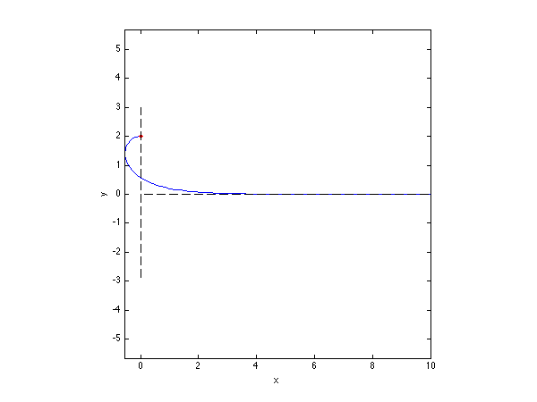
The shape of an overturning meniscus with contact angle -pi/2
Exercices/Contributions
- Please modify this code to compute the shape of a 2D drop hanging below a tap
- Please modify this code for an axisymmetrical hanging drop (you will need to add the additional component of the curvature)