sandbox/easystab/stab2014/brusselator2D_eigenmodes.m
Brusselator 2D - EigenModes and simulation
Coded by Paul Valcke and Luis Bernardos. Simultaneously of us, Guillaume coded the very same version of the Brusselator 2D, his version can be found here. He did an amazingly good job both at solving the problem, explaining it and posing the equations. Rather than repeating the work done by Guillaume, we will focus on what we made different, and on the Eigenmode analysis around a stationnary solution of the flow.
clear all; close all;Parameters
In order to make a “beautiful” and not too much CPU expensive calculation, instead of making a fourier resolution for each march in time, we will use a periodic finite difference scheme. This will allow us increasing the amount of grid points, and then the simulation will be more beautiful.
%%%% parameters
dt = 0.1;
tmax = 30;
Nx=150; % number of grid nodes in x
Ny=150; %number of grid nodes in y
Lx=30;
Ly=30;
k=1;
ka=4.5;
Dparam=8;
mu = 4;
nu= sqrt(1/Dparam);
kbcrit = sqrt(1+ka*nu);
kb = kbcrit*(1+mu);
pts = 3;


% differentiation
[d.x,d.xx,d.wx,x]=dif1D('fp',0,Lx,Nx,pts);
[d.y,d.yy,d.wy,y]=dif1D('fp',0,Ly,Ny,pts);
[D,l,X,Y,Z,I]=dif2D(d,x,y);

% system matrices
NN=Nx*Ny; I2 = speye(2*NN);
E=I2;
A= [D.xx + D.yy - k*(kb+1)*I, Z ;
    k*kb.*I  , Dparam*(D.xx + D.yy)];
b = [k*ka*ones(NN,1);zeros(NN,1)];
% initial condition
C1 = ka.*ones(Nx,Ny);
C2 = (kb/ka).*random('unif',0.99,1.01,[Nx,Ny]); %adds noise
Eigenmodes analysis
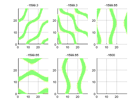
EigenModes
Here we can see the main modes of the brusselator around its stationnary position. We can clearly see several “wave lengths”, that combined will result in the beautiful stripes of the animation at the end of the page.
% We calculate the eigenmodes
[EigenVectors,S]=eigs(A,E);
s=diag(S);  [t,o]=sort(-real(s));
s=s(o); EigenVectors=EigenVectors(:,o);

%Visualisation of the natural modes
figure;
for ind=1:6
    subplot(2,3,ind);
surf(X,Y,reshape(EigenVectors(NN+1:end,ind),Ny,Nx)); shading interp; view(2); axis tight
title(s(ind))
end
drawnow
set(gcf,'paperpositionmode','auto')
print('-dpng','-r100','Bruss2D_EigenModes.jpg')
Resolution
We make a slightly different march in time than Guillaume’s Brusselator.
% march in time matrices
Mm = (E-A*dt/2);
Mp = (E+A*dt/2);

% marching loop
figure;
time = 0;
for time = 0:dt:tmax
    % Calculation of the non-linear term
    fup = k.*C1.^2.*C2;
    fdw = -fup;
    f = [fup(:); fdw(:)];
    q = [C1(:);C2(:)];

    % March in time matrix of non-linear term and b
    Mnl = Mm\((f+b)*dt);%gmres( Mm , ((f+b)*dt), 1000, 1e-7);
    Mlin = Mm\(Mp*q);%gmres( Mm, Mp*q, 1000, 1e-7);

    q=Mlin + Mnl; % one step forward

    C1 = reshape(q(1:NN),Ny,Nx);
    C2 = reshape(q(NN+1:end),Ny,Nx);

    % plotting
    surf(X,Y,C1); shading interp
    axis equal
    view(2);
    title(sprintf('time = %0.02fs of time max = %0.2fs \n\\bf{C1}',time,tmax));
    colorbar;
    xlabel('X');
    ylabel('Y');
    drawnow
    set(gcf,'paperpositionmode','auto')
    print('-dpng','-r80',sprintf('Bruss2D_t%0.1fs.png',time));
end

% Creates animated gif
FirstFrame = true;
gifname = sprintf('Bruss2D_Simul.gif');
for t = 0:2*dt:tmax
   im = imread(sprintf('Bruss2D_t%0.1fs.png',t));
   [imind,cm] = rgb2ind(im,256);
   if FirstFrame
      imwrite(imind,cm,gifname,'gif','Loopcount',inf);
      FirstFrame = false;
   else
       imwrite(imind,cm,gifname,'gif','WriteMode','append',...
           'DelayTime',dt);
   end
end
Result: The animated gif!

Concetration 1 field