sandbox/easystab/stab2014/rayleigh_benard_profil_temperature.m
RAYLEIGH-BENARD INSTABILITY
In this code, we take the code that computes the eigenmodes for free surface waves free_surface_gravity.m and we visualize the flow motion of the first eigenmode of the Rayleigh-Bénard instability based on the resolution of this instability as you can see in rayleigh_benard.m. The Rayleigh-Bénard instability occurs when water or other fluid is heated from below, creating convection cells. We are showing the temperature and velocity fields of the fluid in the convection cells (when yo boil water for example). The top wall is at a cold temperature.
Our system is : \displaystyle \begin{array}{l} \rho u_t=-p_x+ \mu\Delta u,\\t \rho v_t=-p_y+\mu\Delta v-d\rho g \theta,\\ u_x+v_y=0\\ \theta_t+vT_y=\Delta \theta \end{array}
clear all; clf;

n=50;      % number of gridpoints
alpha=2.5;    % wavenumber in x
L=2;        % Fluid height in y
rho=1;      % fluid density
mu=0.001;    % fuid viscosity
g=1;        % gravity
d=1; % thermal dilatation
k=1; % thermal diffusivity
Here, we choose a constant temperature gradient because what we draw in this code are the fluctuations. So, if you want to impose a temperature at the boundaries, you have to choose a gradient. We choose a gradient following the y-axis (we heat the fluid from below).
Ty=-1; % vertical gradient of temperatureEigenmodes of the Rayleigh-Benard instability
Let us use diffusion_eigenmodes.m to calculate the eigenvectors and eigenmodes of our system. By using the differentiation matrices as we learnt from diffmat.m and diffmat_2D.m, we can turn the linear system into a matrix system :
% differentiation matrices
scale=-2/L;
[y,DM] = chebdif(n,2);
D=DM(:,:,1)*scale;
DD=DM(:,:,2)*scale^2;
y=(y-1)/scale;
I=eye(n); Z=zeros(n,n);

% renaming the matrices
dy=D; dyy=DD;
dx=i*alpha*I; dxx=-alpha^2*I;
Delta=dxx+dyy;

% system matrices
A=[mu*Delta, Z, -dx, Z; ...
   Z, mu*Delta, -dy, rho*g*d*I;  ...
   dx, dy, Z, Z;  ...
   Z, -Ty*I, Z, k*Delta];
E=blkdiag(rho*I,rho*I,Z,I);

% boundary conditions
II=eye(4*n); ddy=blkdiag(dy,dy,dy,dy);
u0=1; uL=n; v0=n+1; vL=2*n; T0=3*n+1; TL=4*n;
loc=[u0,uL,v0,vL,T0,TL];
C=[ddy([u0,uL],:); II([v0,vL,T0,TL],:)];
We impose all the fluctuations to 0 in the boundaries.
A(loc,:)=C;
E(loc,:)=0;

% compute eigenmodes
[U,S]=eig(A,E);
s=diag(S);  [t,o]=sort(-real(s)); s=s(o); U=U(:,o);
rem=abs(s)>1000; s(rem)=[]; U(:,rem)=[];
The animation
We show the velocity field and the temperature of the fluid.
%%%%%%%%%%%%%%%%%%%%%%%%%%%%%%%%%%%%%%%%%%%%%%%%%%%%%%%%%%%%%
% velocity and temperature fields figure of the eigenmodes
%%%%%%%%%%%%%%%%%%%%%%%%%%%%%%%%%%%%%%%%%%%%%%%%%%%%%%%%%%%%%

% parameters
nx=100 ;      % number of points in x
You can choose the eigenmode you would like to see here. We chose the 1st one since it’s what we usually see (clouds, boiling water, etc.).
modesel=1;   % which more do animate

% select the eigenmode
u=1:n; v=u+n; p=v+n; teta=p+n;
q=U(:,modesel);
Lx=2*pi/alpha;  x=linspace(-Lx/2,Lx/2,nx);

% expand to physical space

qphys=2*real(q*exp(i*alpha*x));


% add the base flow to the perturbations
uu=qphys(u,:);
vv=qphys(v,:);
We want to show the initial state of the system and its fluctuations. We have to add the initial state of the temperature “theta” to its fluctuations field “qphys(teta,:)”.
[X,Y]=meshgrid(x,y);
Theta=-Y; % imposing the initial state of the temperature to the lower wall
tt=qphys(teta,:)+Theta;

% show the velocity field
sely=1:2:n;
figure(1)
quiver(x,y(sely),uu(sely,:),vv(sely,:),'k'); hold on
surf(x,y,tt,'facealpha',0.5); shading interp;
axis([x(1),x(end),y(1),y(end)]);
xlabel('x'); ylabel('y'); title('Velocity and Temperature field');

% saving the graphic
set(gcf,'paperpositionmode','auto');
print('-dpng','-r80','rayleigh_benard_velocity_temperature.png');
Figures
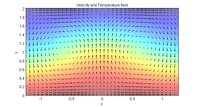
Temperature and Velocity Field
What wee see here is the first eigenmode of the Rayleigh-Bénard instability. We can see the evolution of the temperature of the lower wall which is slowly cooling down. The warm fluid at the bottom, lighter than the cold fluid above, is advected toward the top, while cooling down and getting denser, creating the convection cells. This circle is repeated endlessly.
%}