wave-propagation.c

Inviscid wave propagation in a straight elastic artery
Code
Plots

Inviscid wave propagation in a straight elastic artery

We solve the 1D blood flow equations in a straight artery initially deformed in its center. At t>0, the vessel relaxes towards its steady-state at rest. Consequently, two waves are created that propagate towards both extremeties of the artery. The solution of the flow of blood generated by this elastic relaxation is obtained numerically and compared to the anaytic solution obtained with linear wave theory.

#include "grid/cartesian1D.h"
#include "bloodflow.h"

Geometrical and mechanical parameters.

#define R0 1.
#define A0 pi*R0*R0
#define K0 1.e4
#define L 10.

#define XS 2./5.*L
#define XE 3./5.*L
#define DR 1.e-3

#define C0 sqrt(0.5*K0*sqrt(pi)*R0)

double shape (double x) {

  if (XS <= x && x <= XE)
    return DR/2.*(1. + cos(pi + 2.*pi*(x - XS)/(XE - XS)));
  else
    return 0.;
}

Linear analytic solution for the cross-sectional area A and the flow rate Q.

double analyticA (double t, double x) {
  return A0*pow(1 + 0.5*(shape (x - C0*t) + shape (x + C0*t)), 2.);
}

double analyticQ (double t, double x) {
    return -C0*(-shape (x - C0*t) + shape (x + C0*t))*analyticA(t, x);    
}

Code

int main() {

  origin (0., 0.);
  L0 = L;
  
  riemann = hll_glu;
  
  gradient = order1;
  for (N = 128; N <= 1024; N *= 2)
    run();

  gradient = minmod2;
  for (N = 128; N <= 1024; N *= 2)
    run();

  return 0;
  
}

Initial conditions.

event init (i = 0) {

  foreach() {
    k[] = K0;
    a0[] = A0;
    a[] = a0[]*pow(1. + shape (x), 2.);
    q[] = 0.;
  }
}

Output the computed fields for N=256.

event field (t = {0., 0.01, 0.02, 0.03, 0.04}) {

  if (N == 256) {
    static FILE * fp = fopen ("fields", "w");
    foreach()
      fprintf (fp, "%g %.6f %.6f %.6f %.6f\n", x, a0[], k[], a[], q[]);
    fprintf (fp, "\n\n");
  }
}

event error (t = end) {

  scalar e[];
  foreach()
    e[] = q[] - analyticQ(t, x);

  static FILE * fe = fopen ("errors", "w");
  
  norm n = normf (e);
  fprintf (fe, "%d %g %g %g\n", N, n.avg, n.rms, n.max);
}

Plots


reset

mycolors = "dark-blue red sea-green dark-violet orange black"
mypoints = '1 2 3 4 6 7'

set datafile separator ' '
set style line 1 lt -1 lw 2 lc 'black'

k0 = 1.e4
a0 = pi
c = sqrt(0.5*k0*sqrt(a0))

xi(t, x) = x - c*t
psi(t, x) = x + c*t

xs = 2./5.*10.
xe = 3./5.*10.
dr = 1.e-3

shape(x) = (xs <= x && x <= xe) ? dr/2.*(1. + cos(pi + 2.*pi*(x - xs)/(xe - xs))) : 0.
a(t, x) = a0*(1 + 0.5*(shape (xi(t, x)) + shape (psi(t, x))))**2.
q(t, x) = -c*(-shape (xi(t, x)) + shape (psi(t, x)))*a(t, x)

set output 'A.png'
set xlabel 'x [cm]'
set ylabel 'A [cm^2]'
set key top right

plot a(0., x) w l ls 1 t 'Analytic', \
     a(0.01, x) w l ls 1 notitle, \
     a(0.02, x) w l ls 1 notitle, \
     a(0.03, x) w l ls 1 notitle, \
     a(0.04, x) w l ls 1 notitle, \
     'fields' i 0 u 1:4 every 5 w p lt word(mypoints, 1) lc rgb word(mycolors, 1) ps 2 lw 1 t 't=0', \
     'fields' i 1 u 1:4 every 5 w p lt word(mypoints, 2) lc rgb word(mycolors, 2) ps 2 lw 1 t 't=0.01', \
     'fields' i 2 u 1:4 every 5 w p lt word(mypoints, 3) lc rgb word(mycolors, 3) ps 2 lw 1 t 't=0.02', \
     'fields' i 3 u 1:4 every 5 w p lt word(mypoints, 4) lc rgb word(mycolors, 4) ps 2 lw 1 t 't=0.03', \
     'fields' i 4 u 1:4 every 5 w p lt word(mypoints, 5) lc rgb word(mycolors, 5) ps 2 lw 1 t 't=0.04'

Spatial evolution of the cross-sectional area A computed at $t= (script) {0, 0.01, 0.02, 0.03, 0.04}


set output 'Q.png'
set xlabel 'x [cm]'
set ylabel 'Q [cm^3/s]'
set key top left

plot q(0., x) w l ls 1 t 'Analytic', \
     q(0.01, x) w l ls 1 notitle, \
     q(0.02, x) w l ls 1 notitle, \
     q(0.03, x) w l ls 1 notitle, \
     q(0.04, x) w l ls 1 notitle, \
     'fields' i 0 u 1:5 every 5 w p lt word(mypoints, 1) lc rgb word(mycolors, 1) ps 2 lw 1 t 't=0', \
     'fields' i 1 u 1:5 every 5 w p lt word(mypoints, 2) lc rgb word(mycolors, 2) ps 2 lw 1 t 't=0.01', \
     'fields' i 2 u 1:5 every 5 w p lt word(mypoints, 3) lc rgb word(mycolors, 3) ps 2 lw 1 t 't=0.02', \
     'fields' i 3 u 1:5 every 5 w p lt word(mypoints, 4) lc rgb word(mycolors, 4) ps 2 lw 1 t 't=0.03', \
     'fields' i 4 u 1:5 every 5 w p lt word(mypoints, 5) lc rgb word(mycolors, 5) ps 2 lw 1 t 't=0.04'

Spatial evolution of the flow rate Q computed at $t= (script) {0, 0.01, 0.02, 0.03, 0.04}


set xtics 128,2,1024
set logscale
set cbrange[1e-10:1e10]

ftitle(a,b) = sprintf('Order %4.2f', -b)
f1(x) = a1 + b1*x
f2(x) = a2 + b2*x
f3(x) = a3 + b3*x
f4(x) = a4 + b4*x
f5(x) = a5 + b5*x
f6(x) = a6 + b6*x

fit f1(x) 'errors' every ::0::3 u (log($1)):(log($2)) via a1, b1
fit f2(x) 'errors' every ::0::3 u (log($1)):(log($3)) via a2, b2
fit f3(x) 'errors' every ::0::3 u (log($1)):(log($4)) via a3, b3
fit f4(x) 'errors' every ::4::7 u (log($1)):(log($2)) via a4, b4
fit f5(x) 'errors' every ::4::7 u (log($1)):(log($3)) via a5, b5
fit f6(x) 'errors' every ::4::7 u (log($1)):(log($4)) via a6, b6

set output 'errorQ.png'
set xlabel 'N'
set ylabel 'Error norms'
set key top right

plot "errors" every ::0::3 u 1:2 w p lt word(mypoints, 1) lc rgb word(mycolors, 1) ps 3 lw 2 t '|Q|_1, '.ftitle(a1, b1), \
     exp (f1(log(x))) ls 1 notitle, \
     "errors" every ::0::3 u 1:3 w p lt word(mypoints, 2) lc rgb word(mycolors, 2) ps 3 lw 2 t '|Q|_2, '.ftitle(a2, b2), \
     exp (f2(log(x))) ls 1 notitle, \
     "errors" every ::0::3 u 1:4 w p lt word(mypoints, 3) lc rgb word(mycolors, 3) ps 3 lw 2 t '|Q|_{max}, '.ftitle(a3, b3), \
     exp (f3(log(x))) ls 1 notitle, \
     "errors" every ::4::7 u 1:2 w p lt word(mypoints, 4) lc rgb word(mycolors, 4) ps 3 lw 2 t '|Q|_1, '.ftitle(a4, b4), \
     exp (f4(log(x))) ls 1 notitle, \
     "errors" every ::4::7 u 1:3 w p lt word(mypoints, 5) lc rgb word(mycolors, 5) ps 3 lw 2 t '|Q|_2, '.ftitle(a5, b5), \
     exp (f5(log(x))) ls 1 notitle, \
     "errors" every ::4::7 u 1:4 w p lt word(mypoints, 6) lc rgb word(mycolors, 6) ps 3 lw 2 t '|Q|_{max}, '.ftitle(a6, b6), \
     exp (f6(log(x))) ls 1 notitle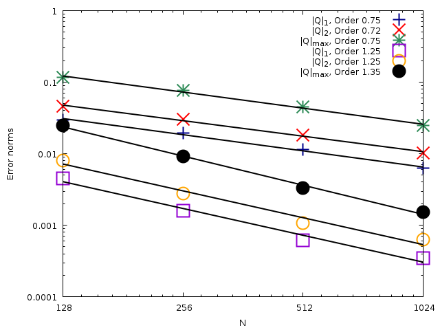

Comparison of the evolution of the error norms for the flow rate Q with the number of cells N. (script)