cylinder-oscillating.c

In-line oscillating cylinder in a quiescent flow at Re = 100 and KC = 5

In-line oscillating cylinder in a quiescent flow at Re = 100 and KC = 5

This test case is inspired from the experiments and numerical simulations of Dutsch et al., 1998. They studied the flow induced by the harmonic displacement in the x-direction of a circular cylinder in an otherwise quiescent fluid for different particle Reynolds numbers Re and different Keulegan-Carpenter numbers KC.

This test case was also reproduced numerically by Guilmineau et al., 2002, Kim et al., 2006, Seo et Mittal, 2011, Orley et al., 2015 and Xin et al., 2018, using the following numerical parameters:

	Re=100, KC=5	Re=200, KC=10
Dutsch et al., 1998	\frac{U_{\infty}\Delta t}{D} \geq 1.1e^{-3}, \frac{D}{\Delta} = 30	\frac{U_{\infty}\Delta t}{D} \geq 2.2e^{-3}, \frac{D}{\Delta} = 30
Guilmineau et al., 2002	\frac{U_{\infty}\Delta t}{D} = 2e^{-3}, \frac{D}{\Delta} = 30?	NA
Kim et al., 2006	\frac{U_{\infty}\Delta t}{D} = ?, \frac{D}{\Delta} = 30	NA
Seo et al., 2011	\frac{U_{\infty}\Delta t}{D} = ? (CFL=0.53), \frac{D}{\Delta} = 60	NA
Orley et al., 2015	\frac{U_{\infty}\Delta t}{D} = ?, \frac{D}{\Delta} \geq 20?	NA
Xin et al., 2018	\frac{U_{\infty}\Delta t}{D} = 1e^{-2}, \frac{D}{\Delta} = 14, 28	NA

We solve here the Navier-Stokes equations and add the cylinder using an embedded boundary.

#include "grid/quadtree.h"
#include "../myembed.h"
#include "../mycentered.h"
#include "../myembed-moving.h"
#include "../myperfs.h"
#include "view.h"

Reference solution

#define d    (1.)
#if RE // Re = 200
#define p_f  (1./10.)
#define Re   (200.)
#else // Re = 100
#define p_f  (1./5.)
#define Re   (100.)
#endif // RE
#define uref (1.) // Reference velocity, uref
#define tref (min (1./(p_f), (d)/(uref))) // Reference time, tref

We define the cylinder’s imposed motion.

#define p_acceleration(t,f) (2.*M_PI*(f)*sin(2.*M_PI*(f)*((t) - 1/(4.*(f))))) // Particle acceleration
#define p_velocity(t,f)     (-cos(2.*M_PI*(f)*((t) - 1/(4.*(f))))) // Particle velocity
#define p_displacement(t,f) (-0.5/M_PI/(f)*sin(2.*M_PI*(f)*((t) - 1/(4.*(f))))) // Particle displacement

We also define the shape of the domain.

#define cylinder(x,y) (sq (x) + sq (y) - sq ((d)/2.))

void p_shape (scalar c, face vector f, coord p)
{
  vertex scalar phi[];
  foreach_vertex()
    phi[] = (cylinder ((x - p.x), (y - p.y)));
  boundary ({phi});
  fractions (phi, c, f);
  fractions_cleanup (c, f,
		     smin = 1.e-14, cmin = 1.e-14);
}

Setup

We need a field for viscosity so that the embedded boundary metric can be taken into account.

face vector muv[];

We define the mesh adaptation parameters.

#define lmin (5) // Min mesh refinement level (l=5 is 2pt/d)
#define lmax (9) // Max mesh refinement level (l=9 is 32pt/d)
#define cmax (1.e-2*(uref)) // Absolute refinement criteria for the velocity field

int main ()
{

The domain is 16\times 16.

  L0 = 16.;
  size (L0);
  origin (-L0/2., -L0/2.);

We set the maximum timestep.

  DT = 1.e-2*(tref);

We set the tolerance of the Poisson solver.

  TOLERANCE    = 1.e-6; // 1.e-14 to test conservation
  TOLERANCE_MU = 1.e-6*(uref);

We initialize the grid.

  N = 1 << (lmin);
  init_grid (N);
  
  run();
}

Boundary conditions

We give boundary conditions for the face velocity to “potentially” improve the convergence of the multigrid Poisson solver.

uf.n[left]   = 0;
uf.n[right]  = 0;
uf.n[bottom] = 0;
uf.n[top]    = 0;

Properties

event properties (i++)
{
  foreach_face()
    muv.x[] = (uref)*(d)/(Re)*fm.x[];
  boundary ((scalar *) {muv});
}

Initial conditions

event init (i = 0)
{

We set the viscosity field in the event properties.

  mu = muv;

We use “third-order” face flux interpolation.

#if ORDER2
  for (scalar s in {u, p, pf})
    s.third = false;
#else
  for (scalar s in {u, p, pf})
    s.third = true;
#endif // ORDER2

We use a slope-limiter to reduce the errors made in small-cells.

#if SLOPELIMITER
  for (scalar s in {u, p, pf}) {
    s.gradient = minmod2;
  }
#endif // SLOPELIMITER
  
#if TREE

When using TREE and in the presence of embedded boundaries, we should also define the gradient of u at the cell center of cut-cells.

#endif // TREE

We initialize the embedded boundary.

We first define the particle’s initial position.

  p_p.x = (p_displacement (0., (p_f)));
  
#if TREE

When using TREE, we refine the mesh around the embedded boundary.

  astats ss;
  int ic = 0;
  do {
    ic++;
    p_shape (cs, fs, p_p);
    ss = adapt_wavelet ({cs}, (double[]) {1.e-30},
			maxlevel = (lmax), minlevel = (1));
  } while ((ss.nf || ss.nc) && ic < 100);
#endif // TREE
  
  p_shape (cs, fs, p_p);

We initialize the particle’s speed and accelerating.

  p_au.x = (p_acceleration (0., (p_f)));
  p_u.x  = (p_velocity     (0., (p_f)));
}

Embedded boundaries

The cylinder’s position is advanced to time t + \Delta t.

event advection_term (i++)
{
  p_au.x = (p_acceleration (t + dt, (p_f)));
  p_u.x  = (p_velocity     (t + dt, (p_f)));
  p_p.x  = (p_displacement (t + dt, (p_f)));
}

#if TREE
event adapt (i++)
{
  adapt_wavelet ({cs,u}, (double[]) {1.e-2,(cmax),(cmax)},
  		 maxlevel = (lmax), minlevel = (1));

We do not need here to reset the embedded fractions to avoid interpolation errors on the geometry as the is already done when moving the embedded boundaries. It might be necessary to do this however if surface forces are computed around the embedded boundaries.

}
#endif // TREE

Outputs

event logfile (i++; t <= 7.5/(p_f))
{
  coord Fp, Fmu;
  embed_force (p, u, mu, &Fp, &Fmu);

  double CD = (Fp.x + Fmu.x)/(0.5*sq ((uref))*(d));
  double CL = (Fp.y + Fmu.y)/(0.5*sq ((uref))*(d));

  fprintf (stderr, "%g %g %d %g %g %d %d %d %d %d %d %g %g %g %g %g %g\n",
	   (Re), (p_f),
	   i, t/(1./(p_f)), dt/(1./(p_f)),
	   mgp.i, mgp.nrelax, mgp.minlevel,
	   mgu.i, mgu.nrelax, mgu.minlevel,
	   mgp.resb, mgp.resa,
	   mgu.resb, mgu.resa,
	   CD, CL);
  fflush (stderr);
}

We also check the mass conservation of the numerical method.

event end_timestep (i++)
{
  double div = 0.;
  foreach (reduction(+:div)) {
    foreach_dimension()
      div += (uf.x[1] - uf.x[])*pow (Delta, dimension - 1);
    if (cs[] > 0. && cs[] < 1.) {
      coord b, n;
      double area = embed_geometry (point, &b, &n);
      foreach_dimension() {
	bool dirichlet = true;
	double ufb = area*(uf.x.boundary[embed] (point, point, uf.x, &dirichlet));
	assert (dirichlet);
	div += ufb*n.x*pow (Delta, dimension - 1);  
      }
    }	
  }
  
  char name2[80];
  sprintf (name2, "div.dat");
  static FILE * fp = fopen (name2, "w");
  fprintf (fp, "%d %g %g %g\n",
	   i, t/(1./(p_f)), dt/(1./(p_f)),
	   div);
  fflush (fp);
}

Snapshots

event snapshot (t = {1./(p_f)*(6.25), 1./(p_f)*(6.25 + 96./360.),
		     1./(p_f)*(6.25 + 192./360.), 1./(p_f)*(6.25 + 288./360.)})
{
  int phase = max(0, floorf ((t/(1./(p_f)) - 6.25)*360));
  
  scalar omega[];
  vorticity (u, omega);
  
  char name2[80];

We first plot the entire domain.

  view (fov = 20, camera = "front",
	tx = 0., ty = 0.,
	bg = {1,1,1},
	width = 800, height = 800);

  draw_vof ("cs", "fs", lw = 5);
  cells ();
  sprintf (name2, "mesh-phi-%d.png", phase);
  save (name2);
    
  draw_vof ("cs", "fs", filled = -1, lw = 5, fc = {1,1,1});
  squares ("u.x", map = cool_warm);
  sprintf (name2, "ux-phi-%d.png", phase);
  save (name2);

  draw_vof ("cs", "fs", filled = -1, lw = 5, fc = {1,1,1});
  squares ("u.y", map = cool_warm);
  sprintf (name2, "uy-phi-%d.png", phase);
  save (name2);

  draw_vof ("cs", "fs", filled = -1, lw = 5, fc = {1,1,1});
  squares ("p", map = cool_warm);
  sprintf (name2, "p-phi-%d.png", phase);
  save (name2);

  draw_vof ("cs", "fs", filled = -1, lw = 5, fc = {1,1,1});
  squares ("omega", map = cool_warm);
  sprintf (name2, "omega-phi-%d.png", phase);
  save (name2);

We then zoom on the cylinder.

#if RE // Re = 200
  view (fov = 9, camera = "front",
	tx = 0., ty = 0., bg = {1,1,1},
	width = 800, height = 600);
#else // Re = 100
  view (fov = 6, camera = "front",
	tx = 0., ty = 0., bg = {1,1,1},
	width = 800, height = 600);
#endif // RE

  draw_vof ("cs", "fs", lw = 5);
  cells ();
  sprintf (name2, "mesh-zoom-phi-%d.png", phase);
  save (name2);

  draw_vof ("cs", "fs", filled = -1, lw = 5, fc = {1,1,1});
  squares ("u.x", map = cool_warm);
  sprintf (name2, "ux-zoom-phi-%d.png", phase);
  save (name2);

  draw_vof ("cs", "fs", filled = -1, lw = 5, fc = {1,1,1});
  squares ("u.y", map = cool_warm);
  sprintf (name2, "uy-zoom-phi-%d.png", phase);
  save (name2);

  stats stp = statsf (p);  
  draw_vof ("cs", "fs", filled = -1, lw = 5, fc = {0,0,0});
  squares ("p", map = cool_warm);
  isoline ("p", n = 20, min = stp.min, max = stp.max);
  sprintf (name2, "p-zoom-phi-%d.png", phase);
  save (name2);

  draw_vof ("cs", "fs", filled = -1, lw = 5, fc = {0,0,0});
  squares ("omega", map = cool_warm);
  isoline ("omega", n = 30, min = -20, max = 20);
  sprintf (name2, "omega-zoom-phi-%d.png", phase);
  save (name2);
}

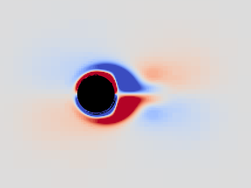
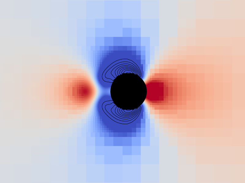
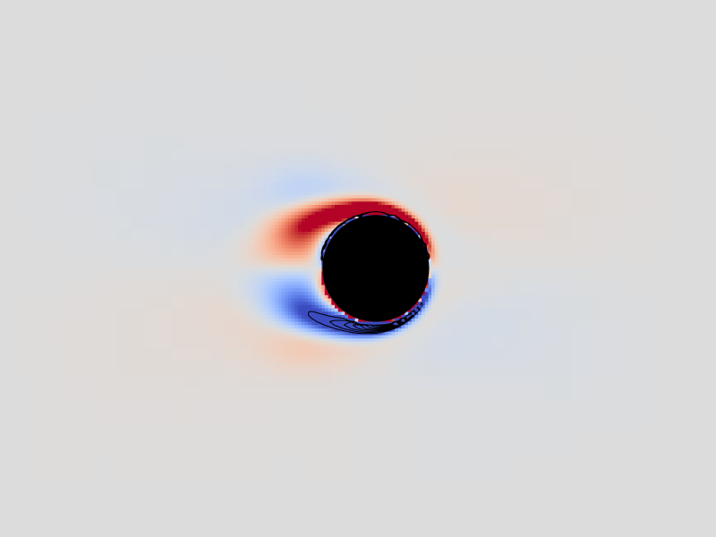
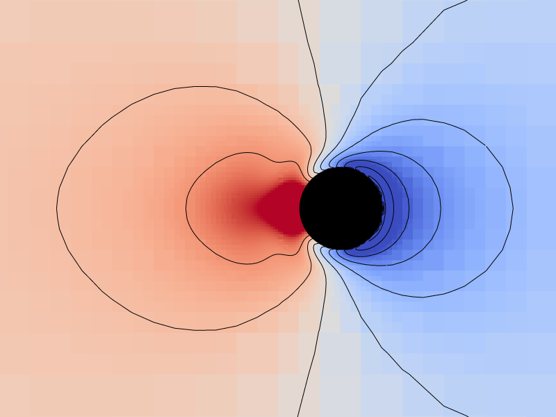
Results

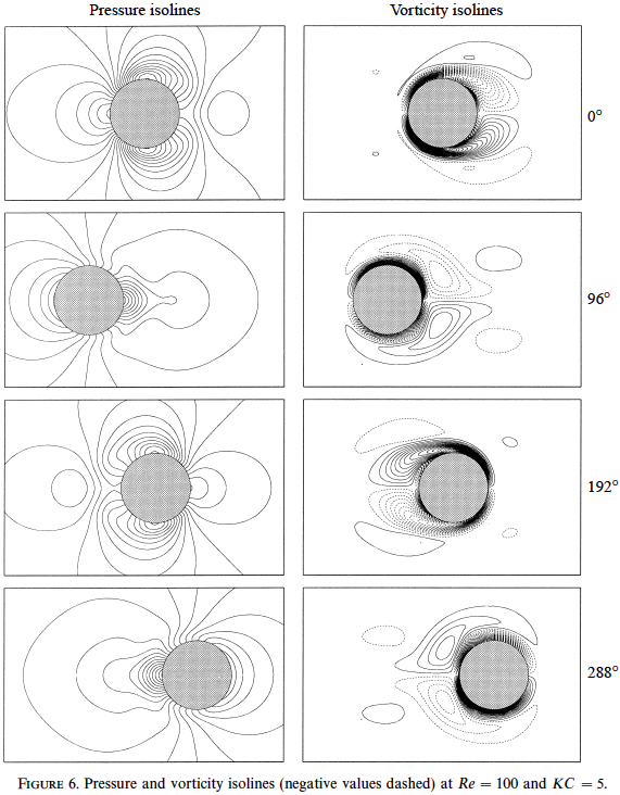
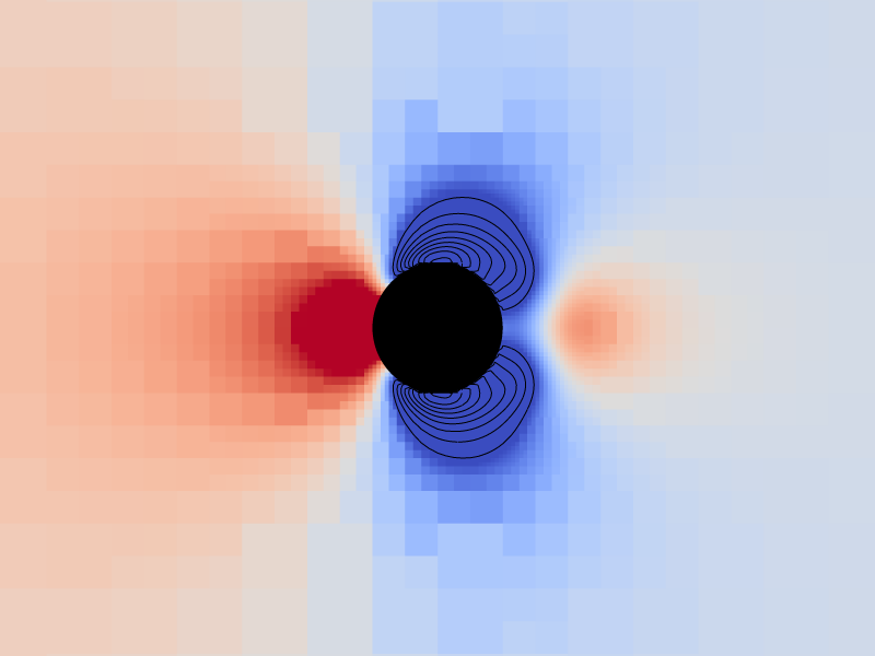
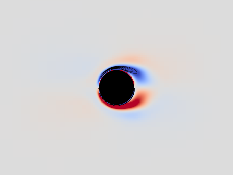
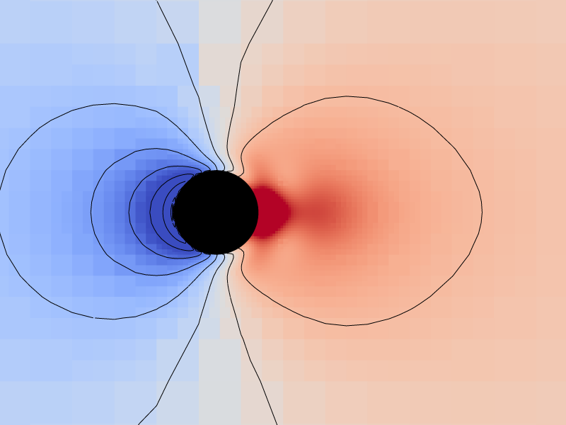
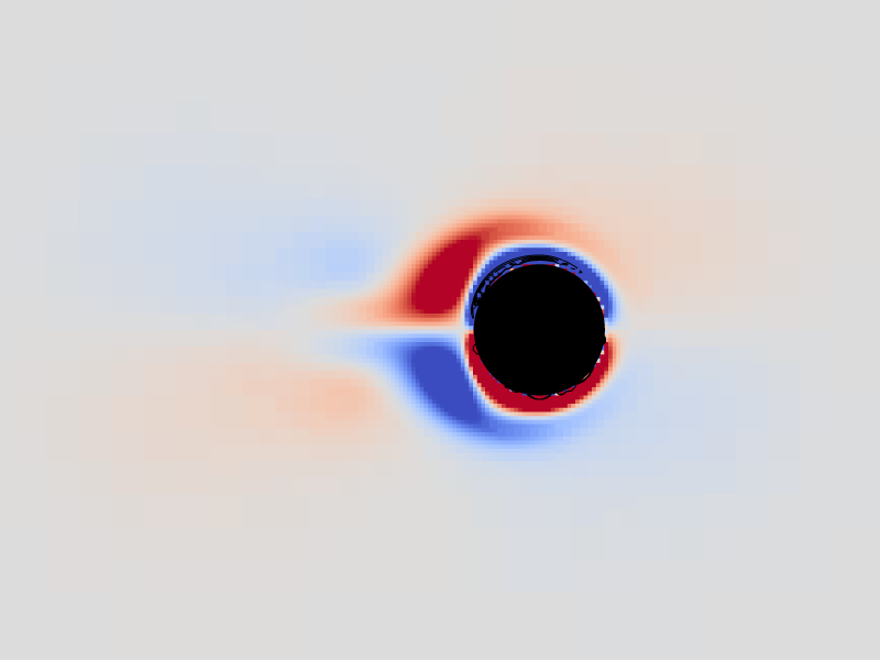
Pressure and vorticity isolines for level = 9

We compare here the pressure and vorticity isolines with those of fig. 6 from Dutsch et al.,1998.

drawing

drawing drawing
drawing drawing
drawing drawing
drawing drawing

Periodicity

We first plot the time evolution of the drag and lift coefficients and verify that the flow has reached a periodic state after 6 cycles.

set terminal svg font ",16"
set key top right spacing 1.1
set xlabel 't/T'
set ylabel 'C_D'
set xrange [0:7.5]
set yrange [-5:8]
plot 'log' u 4:16 w l lw 2 lc rgb "blue" t "Basilisk, l=9"

Time evolution of the drag coefficient C_D (script)

set ylabel 'C_L'
set yrange [-2.5:4]
plot 'log' u 4:17 w l lw 2 lc rgb "blue" t "Basilisk, l=9"

Time evolution of the lift coefficient C_L (script)

set ylabel "dt/T"
set yrange [1.e-4:1e0]
set logscale y
plot 'log' u 4:5 w l lw 2 lc rgb 'blue' t 'Basilisk, l=9'

$Time evolution of the timestep \Delta t (script)$

Time evolution of the timestep \Delta t (script)

Comparison with the results of fig. 10, 15 and 16 from Dutsch et al., 1998

We now plot the time evolution of the drag and lift coefficients over the 6th cycle and compare them with those of of fig. 10, 15 and 16 from Dutsch et al., 1998.

set ylabel "C_D"
set xrange [0:1]
set yrange [-5:7]
unset logscale
plot '../data/Dutsch1998/Dutsch1998-fig10.csv' u 1:($2/0.5) w p ps 0.7 pt 6 lc rgb "black" t 'fig. 10, Dutsch et al., 1998, Re=100 and KC=5', \
     '../data/Dutsch1998/Dutsch1998-fig15-cycle14.csv' u 1:($2/4/0.5) w p ps 0.7 pt 4 lc rgb "black" t 'fig. 15, Dutsch et al., 1998, Re=200 and KC=10', \
     'log' u ($4 - 6.25):16 w l lw 2 lc rgb "blue" t "Basilisk, l=9"

Time evolution of the drag coefficient C_D over the 6th cycle (script)

set ylabel 'C_L'
set yrange [-2.5:4]
plot '../data/Dutsch1998/Dutsch1998-fig16-cycle14.csv' u 1:($2/4/0.5) w p ps 0.7 pt 4 lc rgb "black" t 'fig. 16, Dutsch et al., 1998, Re=200 and KC=10', \
     'log' u ($4 - 6.25):17 w l lw 2 lc rgb "blue" t "Basilisk, l=9"

Time evolution of the lift coefficient C_L over the 6th cycle (script)

Incompressibility with moving boundaries

set ytics format "%.0e" 1.e-20,1.e2,1.e0
set ylabel "div"
set xrange [0:7.5]
set yrange [1.e-20:1.e-4]
set logscale y
plot 'div.dat' u 2:4 w l lw 2 lc rgb 'blue' t 'Basilisk, l=9'

Time evolution of the divergence$ (script)

References

[xin2018]	J. Xin, F. Shi, Q. Jin, and C. Lin. A radial basis function based ghost cell method with improved mass conservation for complex moving boundary flows. Computers & Fluids, 176:210–225, 2018.
[orley2015]	F. Orley, V. Pasquariello, S. Hickel, and N.A. Adams. Cut-element based immersed boundary method for moving geometries in compressible liquid flows with cavitation. Journal of Computational Physics, 283:1–2, 2015.
[seo2011]	J.H. Seo and R. Mittal. A sharp-interface immersed boundary method with improved mass conservation and reduced spurious pressure oscillations. Journal of Computational Physics, 230:7347–7363, 2011.
[kim2006]	D. Kim and H. Choi. Immersed boundary method for flow around an arbitrarily moving body. Journal of Computational Physics, 212:662–680, 2006.
[guilmineau2002]	E. Guilmineau and P. Queutey. A numerical simulation of vortex shedding from an oscillating circular cylinder. Journal of Fluids and Structures, 16:773–794, 2002.
[dutsch1998]	H. Dutsch, F. Durst, S. Becker, and H. Lienhart. Low-reynolds-number flow around an oscillating circular cylinder at low keulegan-carpenter numbers. Journal of Fluid Mechanics, 360:249–271, 1998.