uf.c

Stability of the embedded face velocity interpolation

Stability of the embedded face velocity interpolation

If a “naive” face interpolation is used (by the face_value() macro) to compute face velocities in the centered Navier–Stokes solver, an instability can appear, due to the amplifications of velocity perturbations by the third-order Dirichlet interpolation used to compute viscous fluxes.

This problem is avoided by using an embedded-fraction-weighted interpolation of the face velocities (see /src/embed.h).

#include "grid/multigrid.h"
#include "../myembed.h"

#if NOAVG
#undef cs_avg
#define cs_avg(a,i,j,k)		\
  ((a[i,j,k] + a[i-1,j,k])/	\
   (2.))
#endif // NOAVG

#include "../mycentered.h"
#include "view.h"

Reference solution

#define h    ((L0)/4.)
#define uref (1.) // Reference velocity
#define tref (2.*(h)/(uref)) // Reference time

We define the shape of the domain. We shift the position of the walls by EPS in order for the embedded boundaries not to systematically coincide exactly with the face of a cell. The convergence of the poisson solver for the velocity is sensitive to this value.

#define EPS (1.e-3)

void p_shape (scalar c, face vector f)
{
  vertex scalar phi[];
  foreach_vertex()
    phi[] = -union (y - (h) - (EPS),
		    - (h) + (EPS) - y);
  fractions (phi, c, f);
  fractions_cleanup (c, f,
		     smin = 1.e-14, cmin = 1.e-14);
}

Setup

We need a field for viscosity so that the embedded boundary metric can be taken into account.

face vector muv[];

We also define a reference velocity field.

scalar un[];

Finally, we define the mesh parameters.

#define lvl (5) // Mid mesh refinement level (l=5 is 16pt/(2h))

int main()
{

The domain is 1\times 1 and periodic.

  L0 = 1.;
  size (L0);
  origin (-L0/2., -L0/2.);

  periodic (left);

We set the maximum timestep.

  DT = 4.e-5*(tref);

We set the tolerance of the Poisson solver.

We also increase the number of minimum iterations to improve the accuracy of the velocity solution (not the convergence of the residual).

  stokes = true;
  TOLERANCE = 1.e-7;
  TOLERANCE_MU = 1.e-7*(uref);
  NITERMIN = 5;

We initialize the grid.

  N = 1 << (lvl);
  init_grid (N);
  
  run();
}

Boundary conditions

Properties

event properties (i++)
{
  foreach_face()
    muv.x[] = fm.x[];
}

Initial conditions

event init (i = 0)
{

We set the viscosity field in the event properties.

  mu = muv;

We use “third-order” face flux interpolation.

  for (scalar s in {u, p})
    s.third = true;

We initialize the embedded boundary.

  p_shape (cs, fs);

We also define the volume fraction at the previous timestep csm1=cs.

  csm1 = cs;

We define the boundary conditions for the velocity.

  u.n[embed] = dirichlet (0);
  u.t[embed] = dirichlet (0);
  p[embed]   = neumann (0);

  uf.n[embed] = dirichlet (0);
  uf.t[embed] = dirichlet (0);

We finally initialize the velocity field using a velocity impulse in the y-direction.

  foreach()
    u.y[] = cs[] ? (uref) : nodata;
}

Embedded boundaries

Outputs

event logfile (i++; i <= 100)
{
  fprintf (stderr, "%d %g %g %d %d %d %d %d %d %.3g %.3g %g %g %g\n",
	   i, t, dt,
	   mgp.i, mgp.nrelax, mgp.minlevel,
	   mgu.i, mgu.nrelax, mgu.minlevel,
	   mgp.resa*dt, mgu.resa,
	   normf(u.x).max, normf(u.y).max, normf(p).max);
}

event profile (t = end)
{
  clear();
  view (fov = 20,
	tx = 0, ty = 0,
	bg = {1,1,1},
	width = 400, height = 400);

  draw_vof ("cs", "fs", filled = -1, lw = 5);
  squares ("u.x", spread = -1, map = cool_warm);
  cells ();
  save ("ux.png");

  draw_vof ("cs", "fs", filled = -1, lw = 5);
  squares ("u.y", spread = -1, map = cool_warm);
  cells ();
  save ("uy.png");

  draw_vof ("cs", "fs", lw = 5);
  squares ("p", spread = -1, map = cool_warm);
  cells ();
  save ("p.png");

#if !NOAVG

We make sure that the velocity is not diverging.

  assert (normf(u.x).max < 1e-3);
  assert (normf(u.y).max < 1e-3);
#endif // !NOAVG
}

Results

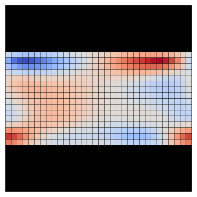
Velocity u.x

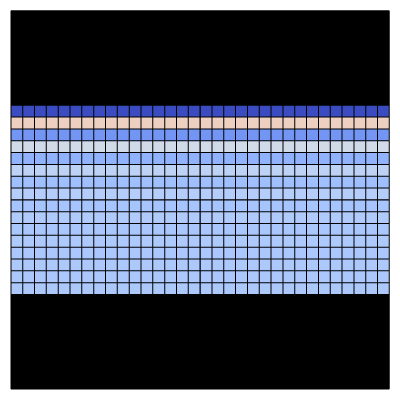
Velocity u.y

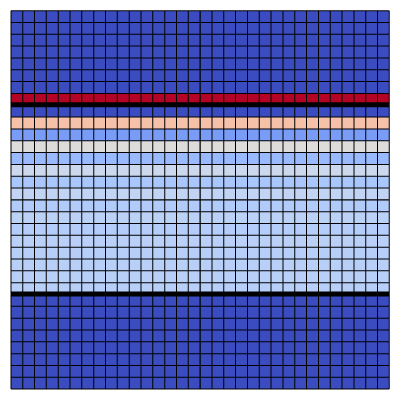
Pressure p

reset
set terminal svg font ",16"
set key top left spacing 1.1
set xtics 0,20,100
set ytics format "%.0e" 1.e-20,1.e-2,1.e2
set xlabel 'n'
set ylabel '||u_x||_{inf}'
set xrange [0:100]
set yrange [1e-8:1e-2]
set logscale y
plot 'log' u 1:12 w l lw 2 lc rgb "black" notitle

Time evolution of the norm of the velocity u_x (script)

set ylabel '||u_y||_{inf}'
plot 'log' u 1:13 w l lw 2 lc rgb "black" notitle

Time evolution of the norm of the velocity u_y (script)