sandbox/gally/KarmanStrouhal.c
Bénard–von Kármán Vortex Street for flow around a cylinder
Re-use of the example code. Modifications to extract velocity and pressure after the cylinder.
We use the centered Navier-Stokes solver, with embedded boundaries and advect the passive tracer f.
#include "embed.h"
#include "navier-stokes/centered.h"
#include "tracer.h"

scalar f[];
scalar * tracers = {f};
double Reynolds;
int maxlevel = 9;
face vector muv[];
The domain is eight units long, centered vertically.
int main() {
  L0 = 8. [1];
  origin (-0.5, -L0/2.);
  N = 512;
  mu = muv;
When using bview we can interactively control the Reynolds number and maximum level of refinement.
  display_control (Reynolds, 10, 1000);
  display_control (maxlevel, 6, 12);

  double Res[] = {
    46.86495177, 50., 59.88745981,
    74.8392283, 99.91961415,
    125., 149.8392283, 174.9196141
  };

  for (int i = 0; i < sizeof(Res)/sizeof(Res[0]); i++) {
    Reynolds = Res[i];
    run();
  }
}
We set a constant viscosity based on the Reynolds number, the cylinder diameter D and the inflow velocity U0.
double D = 0.125, U0 = 1.;

event properties (i++) {
  foreach_face()
    muv.x[] = fm.x[]*D*U0/Reynolds;
}
The fluid is injected on the left boundary with velocity U0. The tracer is injected in the lower-half of the left boundary. An outflow condition is used on the right boundary.
u.n[left]  = dirichlet(U0);
p[left]    = neumann(0.);
pf[left]   = neumann(0.);
f[left]    = dirichlet(y < 0);

u.n[right] = neumann(0.);
p[right]   = dirichlet(0.);
pf[right]  = dirichlet(0.);
The cylinder is no-slip.
u.n[embed] = dirichlet(0.);
u.t[embed] = dirichlet(0.);

event init (t = 0) {

  solid (cs, fs, sqrt(sq(x) + sq(y)) - D/2.);

  foreach()
    u.x[] = cs[] ? U0 : 0.;
}
We check the number of iterations of the Poisson and viscous problems.
event logfile (i++)
  fprintf (stderr, "%d %g %d %d\n", i, t, mgp.i, mgu.i);
We follow the evolution of a point situated after the cylinder.
double xp, yp;

event probe (i++; t <= 35) {

  xp = 0.5*D + 3*D;
  yp = 0.;

  double up = interpolate(u.x, xp, yp);
  double vp = interpolate(u.y, xp, yp);
  double pp = interpolate(p,   xp, yp);

  static FILE * fp = NULL;
  if (!fp) {
    char filename[25];
    snprintf(filename, sizeof(filename), "probe_Re%d.dat", (int)Reynolds);
    fp = fopen(filename, "w");
  }
  fprintf(fp, "%g %g %g %g\n", t, up, vp, pp);
}
We adapt according to the error on the embedded geometry, velocity and tracer fields.
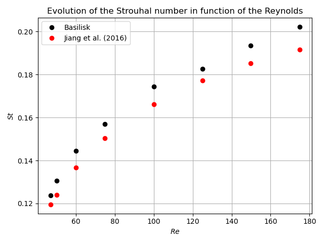
Strouhal number
Reference data from Jiang et al. (2016)
import numpy as np
import matplotlib.pyplot as plt
from scipy.fft import rfft, rfftfreq

# Define problem data
D, U0 = 0.125, 1

# Jiang et al. data
Re_Jiang = [46.86495177, 50, 59.88745981, 74.8392283, 99.91961415, 125, 149.8392283, 174.9196141]
St_Jiang = [0.119480499, 0.123879433, 0.136684722, 0.150366905, 0.166194074, 0.177131267, 0.185232431, 0.191573047]

# Define lists
length = len(Re_Jiang)
St = np.zeros(length)

for i in range(length):

   # Load data: t  vp
   data = np.loadtxt(f"probe_Re{int(Re_Jiang[i])}.dat")
   t  = data[:, 0]
   vp = data[:, 2]

   # Dimensionless data
   time_char = D / U0
   t = t / time_char
   vp = vp / U0

   # Mask (wait until instabilities are established)
   mask = (t > (15/time_char))
   vp = vp[mask]
   t = t[mask]

   vp = vp - np.mean(vp)

   # Time-step
   dt = t[1] - t[0]
   N = len(vp)

   # FFT
   spectrum = rfft(vp)
   freq = rfftfreq(N, d = dt)

   # Strouhal number
   St[i] = freq[np.argmax(np.abs(spectrum))]

plt.plot(Re_Jiang, St, 'ko', label = 'Basilisk')
plt.plot(Re_Jiang, St_Jiang, 'ro', label = 'Jiang et al. (2016)')
plt.xlabel("$Re$")
plt.ylabel("$St$")
plt.title("Evolution of the Strouhal number in function of the Reynolds")
plt.legend()
plt.grid()
plt.tight_layout()
plt.savefig('st-re.png')