diff_test.c

How to use diffusion.h and dr.h together

How to use diffusion.h and dr.h together

This 1D case is an example on how to set boundary condition for a scalar T. Temperature is initialized as an affine function of z, at the surface a (heat) flux is imposed and at the bottom we impose a that the initial gradient is conserved at all t.

#include "grid/multigrid.h"
#include "layered/hydro.h"
#include "layered/nh.h"
#include "layered/remap.h"
#include "layered/perfs.h"
#include "hugoj/lib/diffusionH.h"

double tend = 3600.0;
double smalltime = 1e-10;
double H0 = 100.;
// -> stratification related
double strat = 0.000002;       // [s-2] N^2 stratification
double Ts = 20.;              // [K] Surface temperature (arbitrary)
double qt = -500.;         // [W.m-2] Heat flux
double rho0 = 1025.;     // [kg.m-3] reference density
double cp = 4.2e3;      // [J.kg-1.K-1] heat capacity water
double alphaT = 2e-4;        // [K-1] Thermal expansion coeff for water
double Pr = 1.;                       // Prandtl number = nu/kappa
double kappa = 1.5e-5;         // [m2.s-1] Scalar vertical diffusion coeff
double T0 = 20.;              // [°C] Reference temperature
double Trand = 0.001;           // [°C] Random temperature perturbution
const double g_ = 9.81;        // [m.s-2] Gravity
#define drho(T) (alphaT*(T0-T))       // Linear equation of state (Vallis 2.4)
#define Tini(z) strat/(g_*alphaT)*z + Ts
#include "layered/dr.h"
double fluxbot,fluxtop;



static FILE * fp;

int main(int argc, char *argv[])  
{
  L0 = 50.;
  nu = 0.01;
  kappa = nu;
  N = 1; 
  nl = 30;
  G = 9.81;
  theta_H = 0.51;
  CFL_H = 8.;
  CFL = 0.8;
  
  origin (-L0/2., -L0/2.);

Boundary condition for temperature. We test two cases: i) imposing the initial stratification at top and bottom, ii) impose a destabilising flux at top and initial stratification at bottom.

  fluxbot = strat/(g_*alphaT);
#if HEATING
  fluxtop = qt/(kappa*rho0*cp);
#else
  fluxtop = strat/(g_*alphaT); 
#endif

  #if dimension==2
    periodic (top);
  #endif
  periodic (left);

  run();
}

event init(i =  0) {

  foreach() {
    zb[] = -H0;
    eta[] = 0.;
    double H = - zb[];
    double z = zb[];
    foreach_layer() {
      h[] = H/nl;
      z += h[]/2.;
      foreach_dimension()
        u.x[] = 0.;
      w[] = 0.;
      T[] = Tini(z); // + Trand * noise()*exp(z/100.) ;
      z += h[]/2.;
    }
  }

  fp  = fopen("T_profile.dat","w"); // reset file
  fclose(fp);

}

We impose the stratification at the top and the bottom to be the initial stratification. We should not see any change in the profile.

event viscous_term (i++)
{
  foreach() {
    vertical_diffusion2 (point,   // point
                        h,        // h
                        T,        // scalar
                        dt,       // dt
                        kappa,    // D
                        fluxtop,  // dst
                        fluxbot); // dsb
  }
}

event log (i++){
  fp  = fopen("T_profile.dat","a");
  if (fp == NULL){
    fprintf(stderr, "Error opening file T_profile.dat");
    return 2;
  }
  foreach() {
    foreach_layer()
      fprintf (fp, "%f %d %d %g\n", t, i, point.l, T[]);
  }
  fprintf(fp,"\n\n");
  fclose(fp);
}

event stop (t = tend);

import numpy as np
import matplotlib.pyplot as plt

data = np.loadtxt("T_profile.dat")
nl=30
nt = data.shape[0]//nl

fig, ax = plt.subplots(figsize=(8, 6))
cmap = plt.get_cmap("viridis", nt)
for t in range(nt):
    layer=data[t*nl:(t+1)*nl,2]
    T = data[t*nl:(t+1)*nl,3]
    ax.plot(T,layer,color=cmap(t), marker="+", linestyle="-")
ax.set_xlabel("T")
ax.set_ylabel("Layer")
ax.set_title("Temperature profiles")
ax.set_xlim([19.875,20.025])
#ax.legend(loc="upper left", bbox_to_anchor=(1, 1))
plt.tight_layout()
plt.savefig("T_profiles.png", dpi=150)
plt.show()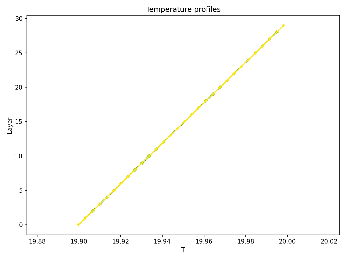

import numpy as np
import matplotlib.pyplot as plt
import os

script_dir = os.path.dirname(os.path.abspath(__file__))
data_path = os.path.join(script_dir, "..", "diff_test_H", "T_profile.dat")

data = np.loadtxt("/home/basilisk-wiki/wiki/sandbox/hugoj/test_diffusion_with_bott_neumann/diff_test_H/T_profile.dat")

nl=30
nt = data.shape[0]//nl

fig, ax = plt.subplots(figsize=(8, 6))
cmap = plt.get_cmap("viridis", nt)
for t in range(nt):
    layer=data[t*nl:(t+1)*nl,2]
    T = data[t*nl:(t+1)*nl,3]
    ax.plot(T,layer,color=cmap(t), marker="+", linestyle="-")
ax.set_xlabel("T")
ax.set_ylabel("Layer")
ax.set_title("Temperature profiles")
ax.set_xlim([19.875,20.025])
#ax.legend(loc="upper left", bbox_to_anchor=(1, 1))
plt.tight_layout()
plt.savefig("T_profiles.png", dpi=150)
plt.show()