sandbox/Antoonvh/The_Tree-Grid_Structure_in_Basilisk

The Tree Grid Structure in Basilisk

Basilisk can use so-called tree-structured grids. These types of grids are used for simulations where the resolution is not constant within the spatial domain. Furthermore, the tree structure provides a convenient and efficient layout for dynamic grid refinement and coarsening. This page discusses the first principles of tree-structured grids as they are used in Basilisk. Note that these grids are used for a wide variety of applications (e.g., data storage).

This page was written to guide the writing of the paper by Van Hooft et al. (2018).

Multigrid

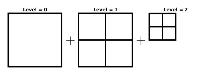
First, the multigrid is discussed: Multigrid is short for ‘Multiple resolution grid’, and is a grid that has more than one spatial resolution. The most rudimentary grid in a two dimensional square domain of size of L_0\times L_0 is a single L_0\times L_0-sized cell. A multi-resolution grid forms when one or more levels of refinement are added. For example, we could also mesh the domain with cells that have double the resolution of the original cell (i.e. \Delta = L_0/2), resulting in a 2\times 2-cell grid. For a multigrid with l levels of refinement, the grid consists of 2^l\times 2^l cells at the maximum resolution.

The Multigrid is a combination of grids at different levels of refinement

Such multigrids are used to speedup iterative solvers such as Basilisk’s Poisson solver. The hierarchic structure in a multigrid can be generalized to a tree grid.

The Tree Grid

A multigrid (as presented above) does not have a variable resolution in the spatial domain. From the figure above we can easily associate all 16 grid cells at the highest level to one of the four cells at one level lower. An obvious way of doing this is exemplified below,

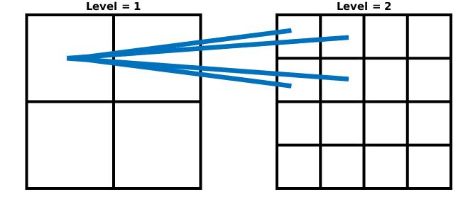
Connecting cells different levels: A parent and its children

The four cells that exist on a higher level are called the ‘children’ of the cell at the lower level. Therefore, the low-level cell is a ‘parent’. The parent cell in this example is also a child, its parent is the root cell. An obvious way of introducing a varying spatial resolution is to not initialize the children of some parents at a given level. For example, we can only initialize the children of the top left cell at Level = 1. The grid would look like this:

The cells within a simple Tree grid

This is what is referred to as a tree grid. With increasing refinement levels, there exist many permutations of possible grid structures. In order to keep track of all the cells we can draw a conceptual picture of the grid shown above:

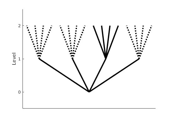
Conceptual view of the tree grid from the example above

This figure reveals part of the etymology of “tree grids”. The figure draws connections between parents and children cells at each level. We see that at level = 2, there are only 4 grid cells originating from a single parent cell at level = 1. The 12 children of the other cells at level = 1 are not defined, indicated by the dashed lines.

Nomenclature, iterators and resolution boundaries

It is possible to iterate trough all cells in a tree using the foreach_cell() iterator. For example if you want to find all the (centered) locations of the cells in your simulation you could use,

foreach_cell()
  fprintf(ferr,"x = %g y = %g\n",x,y); 

The foreach_child iterator can be used to iterate over the children of a given cell. For example, we could count the number of children each cell has by nesting iterators:

foreach_cell() {
  int n = 0; 
  foreach_child()
    n++;
  printf ("%d\t", n);

For an D-dimensional grid, all cells have 2^D children. If you would like to find the value of a scalar field using the foreach_child() iterator, the following code will produce an error:

scalar a[];
...
  foreach_cell() {
    printf ("The value of a in this cell is %g\n", a[]);
    foreach_child()
      printf ("The value of a in this child is %g\n", a[]);
  }
...

The example above will produce an error upon running (it will compile). This error indicates that we have tried to access a non-initialized value as not all cells have children. It is therefore useful to distinguish between the different types of cells within a tree. For every cell one (and only one) of these statements is true:

• All its children are cells (i.e. a simple parent)
• The cell is a leaf and its children are not active
• The cell is a leaf and a halo
• The cell is a child of a halo cell (a Ghost)

We can already understand the first statement. For example, the root cell at level = 0 typically falls in the first category. The second statement introduces the concept of leaf cells: A cell is a leaf when this cell is at the end of a tree branch. For a given point in the domain, the location of this point is typically within multiple cells at different levels. The leaf cell is the cell at the highest level that encompasses this point. It is possible to find the location of a leaf cell for any given location in the domain using locate()

...
Point point = locate (xp, yp);
printf ("x = %g y = %g\n", x, y);
...

Furthermore, because a leaf cell is at the highest level for any given location, they are often the only cells that need to be iterated by the user (why care about some coarser level solution when you have a fine-level solution?). Therefore, the leaf cell iterator is the most commonly used iterator: the foreach() iterator. To find the (centered) locations and the level for each leaf cell in your grid you could do:

...					 
foreach()
  printf"x = %g y = %g level = %d\n", x, y, level);
...

But you probably already knew this from the examples and the tutorial. The third and fourth category use the concept of halo’s. A tree grid facilitates resolution boundaries between leaf cells. As such, a halo is a marked leaf cell at the coarse side of the resolution boundary. Its purpose is to provide a higher-level estimate of the field defined via its children. These children to halo cells themselves are (obviously) of the fourth category. You can cycle trough all halo cells at a certain level l within your grid using the foreach_halo() iterator, like so;

...
int l = 2;
foreach_halo (prolongation, l)
  fprintf(ferr,"x = %g y = %g a = %g\n", x, y, a[]);
...

For virtually all of Basilisk’s applications, there is no need to remember this iterator. By design, it suffices to define a scalar field using the leaf iterator (i.e foreach()). Even tough the parent cells and additional halo cells already exist, the values remain uninitialized they are set. You can ensure that this is the case by calling the boundary() function for: a field a, a list including a and b and all fields. e.g.

...
boundary ({a});
boundary ({a, b});
boundary (all);
...

Not only does the boundary() function define the cell values at the box boundaries of your domain, it also handles the resolution boundaries within the domain. For the latter purpose it employs the interpolation methods defined with the ‘prolongation’ and ‘restriction’ attributes to define values for halo-ghosts and parent cells, respectively. This also explains why users only to care about the leaf-cell solution: The non-leaf-cell values are simply derived from the leaf cell values, and should not have independent information. Note that after calling boundary(), all leaf and parent cells can employ simple Cartesian stencils for computations.

An example grid

Now that we know about cells, leafs and halos we can realize that the example previous example grid does not make much sense. Now look at an example grid that is generated by basilisk itself. Using the following code:

#include "grid/quadtree.h"
int main() {
  L0 = 16;
  X0 = Y0 = 0;
  init_grid (4); // Initialize a 4 x 4 grid
  refine ((x > 12) && (y > 12) && (level < 3)); // Refine to top right corner
  unrefine ((x < 8) && (y < 8) && level >= 1); // Coarsen the bottom left corner
  printf ("#All cells:\n");
  foreach_cell()
    printf ("%d %g %g %g\n", level, x, y, Delta);
  printf ("\n#leafs:\n");
  foreach()
    printf ("%d %g %g %g\n", level, x, y, Delta);
  int i = 1; 
  boundary (all);
  while (i <= depth()){
    fprintf (ferr, "\n#halo ghosts at level %d\n", i);
    foreach_halo (prolongation, i - 1){
      foreach_child(){
        fprintf (ferr, "%d\t%g\t%g\t%g\n", level, x, y, Delta);
      }
    }
    i++;
  }
}

This results in the following grid structure that can be plotted using the output of the script above:

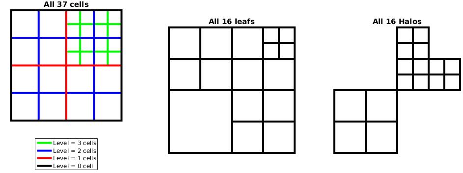
Grid structure generated with the script above (“Halos” should read “Halo Ghosts”)

Also we may draw a tree-structure plot of this grid:

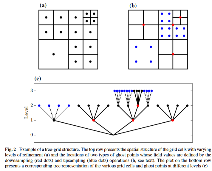
This is figure 2 of Van Hooft et al (2018).

Indexing and MPI load balancing

This section is more conceptually inspired than the text above. The code under grid/tree-mpi.h is not as legible for me.

The leaf cells are iterated sequentially using a so-called N-order space filling curve. We can check what this entails by plotting the output from the script above.

Notice that in this example, the leaf-cell iterator is iterating from coarse to fine level cells. This is coincidence(!) and is typically not the case. You will see another example soon where this “feature” is not present. This N-order indexing method has provided a method to map our 2D grid on to a 1D line. Note that this is not a luxury since the memory addresses on the computer are also ordered linearly.

The N (or Z) order indexing has the favorable property that cells that are close in the 2D space often remain close on the 1D memory axis (does it really?). This is an important feature for the performance of many solvers given that computer systems tend to load the data stored in the RAM-memory in blocks onto the CPU-cache memory. As now (values of) neighboring cells can be accessed without too much calls for communication between RAM and cache. One may watch this excellent movie on youtube to learn a bit more about space filling curves and some of their desirable properties. Can you think of a reason not to use the Hilbert curve from the movie?

Finally, the load balancing between the MPI processes is (conceptually) rather straight forward. Once the grid points are ordered along a line it is really as simple as chopping up the line in N equal parts for N processes. The “close neighbors” property of the curve ensures quite some skill in minimizing the MPI-domain-interface communications. That seems like a rather elegant idea compared to the work of G. Agbaglah et al. (2011).

We can view the the parallel grid iterator in the following movie that is generated on this page.

Noting that by rendering each individual frame of the movie, the cell iterations were synchronized between the threads. It can be useful to keep in mind that this is generally not the case, and that individual threads do their jobs asynchronous for another unless they are explicitly told to do otherwise.

So far we have seen that cells can be associated with resolution boundaries. Also ghost cells at the edge of the domain are present to implement boundary conditions. Furthermore, the MPI-domain decomposition introduces a new type of boundaries. There are cells introduced at the MPI-boundaries to facilitate communication of cell values between the neighboring processes. These are also automatically identified when calling to the boundary() function.

For more info one may read: This work of M. Griebel and G. Zumbusch. I was told parts of it hold true for Basilisk.