front_page.c

The Frontpage for a Thesis.

The Frontpage for a Thesis.

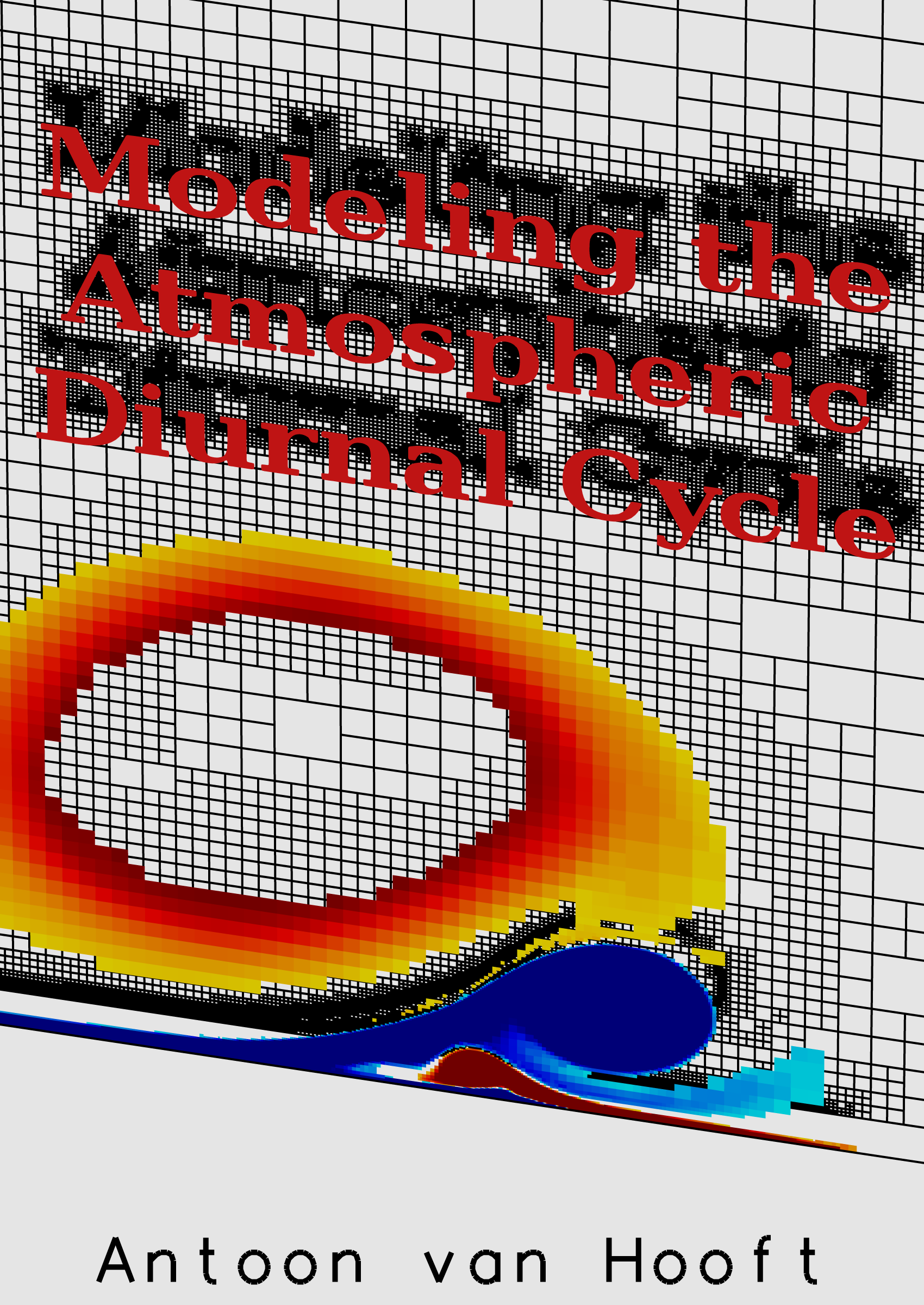
This page is usefull for those who wish to obtain a thesis cover with the title ‘Modeling the diurnal cycle’ and go by the name ‘Antoon van Hooft’.

What?

The cover visualizes vorticity dynamics which are computed with the Navier-Stokes solver. The title’s letters are represented on a tree grid. We follow this test page. Finally, Basilisk view is used to visualize the corresponding tree data.

#include "navier-stokes/centered.h"
#include "distance.h"
#include "fractions.h"
#include "view.h"

The setup follows the setup of the vortex-wall collision, which is governed by a Reynolds number Re,

double Re = 4000.;
u.t[bottom] = dirichlet (0.);

int main() {
  L0 = 15.;
  X0 = -L0/2;
  const face vector muc[] = {1./Re, 1./Re};
  mu = muc;
  run();
}

The flow is initialized with a Lamb-Chaplygin dipolar vortex.

double yo = 5, xo = 0.1;                        //Dipole centre coordinate
#define RAD (pow(sq(x - xo) + sq(y - yo), 0.5)) //r(x,y)
#define ST ((xo - x)/RAD)                       //Sinus of the azimuth angle

event init (t = 0) {
  double k = 3.83170597;
  scalar psi[];
  refine (RAD < 2.0 && level <= 9);
  refine (RAD < 1.0 && level <= 10);
  foreach() 
    psi[] = ((RAD > 1)*((1/RAD))*ST +
	     (RAD <= 1)*(-2*j1(k*RAD)*ST/(k*j0(k)) + RAD*ST));
  boundary ({psi});
  foreach() {
    u.x[] = -((psi[0, 1] - psi[0, -1])/(2*Delta));
    u.y[] = (psi[1, 0] - psi[-1, 0])/(2*Delta);
  }
  boundary({u.x, u.y});
}

We use an adaptive grid.

event adapt (i++)
  adapt_wavelet({u.x, u.y}, (double[]){0.025, 0.025}, 11); // 11

Generate the image

At t = 6 an event is called that outputs the image.

event output_image (t = 6) {
  scalar d[], omega[];

First we load and place the title letters that are stored in the .gnu format and are generated with Inkscape and Gnuplot.

  double ttx = .9, tty = 1.2, ttw = 1.5;
  coord * p;
  coord min, max;
  p = input_xy (fopen ("front_page.title.gnu", "r"));
  bounding_box (p, &min, &max);
  int j = 0;
  double w = max.x - min.x;
  while (p[j].x > 0.1 && p[j].x < 1E6) {      //Reshape
    p[j].x = (p[j].x - min.x)*(ttw/w) + ttx;
    p[j].y = (p[j].y - min.y)*(ttw/w) + tty;
    j++;
  }
  distance (d, p);
  while (adapt_wavelet ({d, u.x, u.y}, (double[]){1e-3, 0.02, 0.02}, 13).nf);
  vertex scalar phi[];
  scalar f[];
  foreach_vertex()
    phi[] = (d[] + d[-1] + d[0,-1] + d[-1,-1])/4.;
  face vector s[];
  fractions (phi, f, s);

Next, The vorticity field is computed and made transparant in some locations.

  vorticity (u, omega);
  foreach()
    if (fabs(omega[]) < 2 || (y > 0.2 && omega[] > 7))
      omega[] = nodata;

The last step is to output a high resolution image with bview commands.

  view (fov = 2.87579, phi = 0.61, theta = 0.25,
	tx = -0.106311, ty = -0.035, bg = {0.9,0.9,0.9},
	width = 1700, height = 2400, samples = 4);       //Set the camera,
  draw_vof ("f", "s", filled = 1, fc = {0.9, 0.1, 0.1}); //print the title,
  squares ("omega", min = -7, max = 7);                  //plot vorticity field,
  begin_translate (z = -0.1);                            //move to the back ground
    cells (lw = 4);                                      //plot the cells,
  end_translate();
  draw_string ("  Antoon van Hooft", size = 20, lw = 10);//add the author's name,
  box (notics = true, lw = 4);                           //And draw a boundary line. 
#if 0                                                    //Flip switch for `raw` output
  save ("front_page.ppm");                               //Save the image
#else
  save ("front_page.png");                               //Possibly compressed
#endif
}

The result

Here is the cover:

Well done bview!